The paired t-test is used to check whether the average differences between two samples are significant or due only to random chance. In contrast with the “normal” t-test, the samples from the two groups are paired, which means that there is a dependency between them.
The following example illustrates the difference between the regular t-test and the paired t-test: Internal customers of an information technology (IT) help desk are asked to rate their satisfaction with the help desk service before and after an improvement project. In a typical t-test situation, practitioners would ask a group of users before the improvement and another, different group of users after; in a paired t-test condition the same users are asked twice, once before and once after the project. The answers before and after are now paired with the same user. A simple way to identify whether the paired t-test is appropriate is to ask the question: Does it make sense to calculate differences between pairs of results?
To use the paired t-test, however, the calculated differences between the two samples must be normally distributed. If this is not the case, the paired t-test cannot be used. Fortunately, it has a nonparametric equivalent: the 1-sample sign test. This is used to compare an observed median with a hypothesized median. It works when the Y variable is continuous, discrete-ordinal or discrete-count.
Looks Can Be Deceiving
A 1-sample sign test may help in determining the meaning behind a data set. An example: A project team wants to compare the number of machine breakdowns of 10 different machines before and after an improvement (see table below).
| Machine Breakdowns Using Standard and New Methods | |||
| Machine | Breakdowns with Standard Processing Method | Breakdowns with New Processing Method | Difference Between Methods |
| 1 | 2 | 2 | 0 |
| 2 | 4 | 2 | -2 |
| 3 | 1 | 3 | 2 |
| 4 | 6 | 4 | -2 |
| 5 | 4 | 4 | 0 |
| 6 | 4 | 2 | -2 |
| 7 | 4 | 2 | -2 |
| 8 | 2 | 2 | 0 |
| 9 | 1 | 3 | 2 |
| 10 | 6 | 4 | -2 |
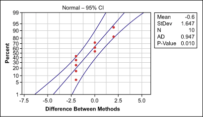
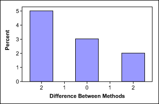
The difference between the standard and the new method is not normally distributed (Figure 1), which is mainly due to too few distinct value categories (Figure 2). Therefore, the team decides to use the 1-sample sign test to determine if the difference is significant or due only to random chance. If there was no difference between the number of breakdowns before and after, the practitioners would expect the median of the differences between the two methods to be equal to zero.
This means that the null hypothesis for the 1-sample sign test is that the observed median is equal to zero, while the alternative hypothesis states that the observed median is not zero.


The output from statistical analysis software (shown below) shows that the observed median is -1, making it appear that the new method reduced the number of breakdowns. The p-value, however, is 0.45. This means that the probability that the median difference between the standard and new method is only randomly different from 0 is still 45 percent. Because this risk is greater than 5 percent, it is not accurate to conclude that there is a significant difference in the number of breakdowns after the improvement.
Sign test of median = 0.00000 versus not = 0.00000
N Below Equal Above P Median
Difference between methods 10 5 3 2 0.4531 -1.000
How It Works
What is interesting about the 1-sample sign test is that it can be used to compare two samples with each other, though by its nature it only compares the observed median of one sample with a hypothesized median. This is because in a paired condition, practitioners actually do not need to compare the medians of the two samples; it is enough to only compare the median of the difference between the two groups. One sample is created by subtracting two samples from each other and comparing this one sample against a hypothesized median (zero in this case).
The test statistics of the 1-sample sign are based on a simple consideration: If the null hypothesis is true (i.e., no difference between the observed and the assumed median of zero), the probability of finding observations above the assumed median should be equal to the probability of finding observations belowthe assumed median. Or, in mathematical terms:
Pobservations below = Pobservations above = 0.5
Therefore, the 1-sample sign test determines the probability (p-value) of observing a specified number of observations above versus below the hypothesized median.
In the example above, five machines had a reduction of breakdowns with the new method (a difference below zero) while two machines had an increase of breakdowns with the new method (a difference above zero). If there was truly no difference between standard and new, we would expect half the machines to be below and half above the median of zero.
The 1-sample sign test now uses the binomial theory to determine the probability that – although assuming no difference – five out of seven (five below + two above) machines show a reduction of breakdowns. This probability is the p-value for the test shown above.
A p-value of 0.45 means that there is a 45 percent chance of five out of seven machines logging a reduction in breakdowns if there actually was no difference between the methods. Therefore, the practitioners cannot reject the null hypothesis and would conclude that the new method does not help to improve the number of breakdowns.