
In the development phase of Design for Six Sigma (DFSS), practitioners who work in domains such as medical devices, pharmaceuticals, foods, material composition and semiconductors frequently deal with experiments to determine optimal ingredient mixtures for desired products. The factors in a mixture experiment are the ingredients or components of a mixture, and the response is a function of the proportion of each ingredient. These proportional amounts of each ingredient are typically measured by weight, volume or mole ratio. Designing, executing and analyzing mixture experiments requires different approaches than those used for factorial experiments.
The following is a step-by-step process for dealing with mixture experiments using an example taken from a Six Sigma project in a medical device industry.
Mixture Design Space
The main distinction between factorial experiments and mixture experiments is the construction of their design space. The design space of a factorial experiment is the set of possible combinations of its independent variables or components. The design space of a mixture experiment is the set of possible combinations of the relative proportion of each component, which usually add up to a certain value. Exploring design space means evaluating the various design options possible with a given technology and optimizing with respect to specific constraints, such as process or amount. Figure 1 illustrates the distinction between factorial design space and mixture design space for three different components.
When the mixture components are subject to the constraint that they must add up to 1, they construct a standard mixture design. The standard mixture design space is shown as a triangle area inside the cube of Figure 1. Simplex-lattice designs and simplexcentroid designs are fitting models for the standard mixture design. When mixture components are subject to additional constraints, such as a maximum or minimum value for each component, they construct a design other than the standard mixture design, referred to as a constrained mixture design. The constrained mixture design space is shown in Figure 1 as a polygonal area in the triangle. Extreme-vertices designs are fitting models for the constrained mixture design.

The main objective in a mixture experimental area is to find the optimal response for any mixture or combination of the components, and to obtain the influence on the response of each component singly and in combination with other components. In mixture experiments, practitioners generally assume that the true underlying response surface is continuous over the space being studied, with no specific trend of its errors.
There are three types of mixtures:
- Mixture of components, which only needs to fit a model for the components, as shown in Figure 1.
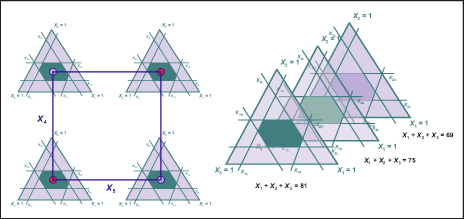
- Mixture-factorial experiments, which need to fit a model for the components and factorial variables. The design space on the left in Figure 2 shows a hydrophilic mixture of three components (x1, x2, x3) at full factorial combinations of two two-level change transfer agents (CTAs) (x4, x5) for a medical device material development.
- Mixture-amount experiments, which need to fit a model for the components and the amount variable. The design space on the right in Figure 2 shows an experiment for three different amounts of the mixture – Tot 1, Tot 2 and Tot 3 units.
Experiment Execution, Logistics and Trade-off Issues
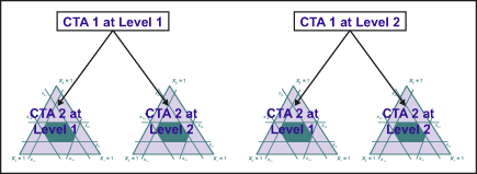
Many industrial experiments restrict randomization due to limited resources or economical considerations. For example, the levels of hard-to-change variables are held fixed, while all the combinations of the other variables are run. This is illustrated in Figure 3, where levels of CTA 1 are held fixed and CTA 2 is varied for all the combinations. This leads to more complex models, such as split-plot design and analysis because it introduces two sources of experimental error.
Logistics of an experiment often make data collection more complicated. For example, because a certain medical device material synthesis needs a long process, but the product launch date is fixed, there is a desire to reduce the number of experiments to be performed, while still being able to investigate many factors simultaneously.
Rarely does a product have simply a single response. Optimizing a product with multiple responses is in many cases a trade-off issue. For example, medical device material development addresses trade-off issues involving the modulus of elasticity, resistance to optical defects and tearing, water rinse-ability, surface wet-ability, water content at ambient temperature, and oxygen permeability at 35 degrees Celsius.
To discover optimal and robust formulations within limited resources, practitioners need to have an experimentation strategy that imposes a sequentially true design of experiments in all experimentation. In other words, the mainexperiment consists of a sequence of subexperiments, each depending on the statistical analysis based outcome of the previous one. If n such subexperiments are chained, then the full experiment results in a chain of events, or a path.
Steps in Mixture Designs
A project involving the development of new medical device material can be used to show steps in planning and analyzing experiments with mixtures using statistical analysis software.
Step 1: Define the Objectives of the Experiment
The objective of the experiment in this project is to find the best ingredient to get optimal medical device materials in terms of its modulus and water content (% H2O) at ambient temperature.
Step 2: Select the Mixture Components and Any Other Factors to Be Studied
Practitioners fix other ingredients for making medical device materials except three main components: Monomer A, Monomer B and Monomer C. A monomer is a small molecule that may become chemically bonded to other monomers to form a polymer, or plastic, for medical device materials.
Step 3: Identify Constraints in Order to Specify the Experimental Region
The total percentage of each monomer used in a mixture must be in the following range:
Min A percent < A < Max A percent
Min B percent < B < Max B percent
Min C percent < C < Max C percent
Based on previous historical data, practitioners now need to further observe mixtures at three different amounts: A + B + C = Total 1 percent, Total 2 percent and Total 3 percent of the total medical device materials.
Step 4: Identify the Response Varaibles and Their Targets
Two out of several responses used in this example are Young’s modulus of the material elasticity (expressed in megapascals [MPa]) and the water content of the medical devices. The functionality of the modulus and the water content are related to comfort, one of the most desirable qualities for medical device wearers. In this example, the target of the modulus is 0.75 MPa and the water content is 35 percent.
Step 5: Propose an Appropriate Model
The practitioners propose that it is enough to fit a linear model with linear interactions between monomers and three different amounts of formulation to the response data. This can be done using lattice degree 1.
Step 6: Select an Experimental Design that is Sufficient to Fit the Proposed Model
Because the mixture components are constrained, the practitioners apply extreme-vertices designs to create their design space. To get a better understanding of the behavior of the medical device material responses at the middle design space (Total 2 percent), practitioners need to add center and axial points. They also add a center point of the design space at the material total percentages of Total 1 percent and Total 3 percent. The design points at the three different amounts are shown in Figure 4. The coded value of each design point is tabulated in the first three columns of Table 1.

Step 7: Collect Experimental Data and Determine Feasible Design Space
Once the experimental design matrix and logistics are set, practitioners can run the experiment to collect data. Experimental results are shown in the last two columns of Table 1. Feasible design space is the set of possible designs and design parameters that meet specific product requirements. The feasible design spaces with specs of a modulus between 0.7 MPa and 0.8 MPa and water content between 32 percent and 38 percent for three different amounts are shown as white areas in Figure 5. Clearly, not all of the experimental results shown in Table 1 fall into the feasible space.
| Table 1: Design Matrix and Its Responses | |||||
| A (%) | B (%) | C (%) | Total Ingredients (%) | Modulus (MPa) | %H20 |
| A2 | B2 | C11 | Total 2 | 0.56 | 29.6 |
| A2 | B11 | C2 | Total 2 | 0.88 | 44.85 |
| A6 | B6 | C6 | Total 2 | 0.81 | 35.35 |
| A4 | B4 | C9 | Total 2 | 0.61 | 32.65 |
| A9 | B4 | C4 | Total 2 | 0.88 | 32 |
| A11 | B2 | C2 | Total 2 | 0.96 | 32.07 |
| A4 | B9 | C4 | Total 2 | 0.94 | 41.09 |
| A2 | B7 | C8 | Total 2 | 0.75 | 39.2 |
| A7 | B7 | C2 | Total 2 | 0.99 | 38.05 |
| A7 | B2 | C8 | Total 2 | 0.8 | 30.65 |
| A12 | B9 | C3 | Total 3 | 1.11 | 31.6 |
| A5 | B7 | C3 | Total 3 | 0.9 | 45.35 |
| A5 | B12 | C12 | Total 3 | 0.6 | 30.9 |
| A8 | B8 | C7 | Total 3 | 0.9 | 35.9 |
| A10 | B1 | C1 | Total 1 | 1.02 | 29.7 |
| A1 | B10 | C1 | Total 1 | 0.85 | 43.75 |
| A1 | B1 | C10 | Total 1 | 0.52 | 31 |
| A3 | B3 | C5 | Total 1 | 0.78 | 35.45 |

Step 8: Analyze the Influence of Each Design Variable
First, practitioners observe the total influence of all components and the total influence of the linear interaction between monomers and formulation amounts. This can be done by using an analysis of variance (ANOVA)-based regression method (Figure 6). R2 of the linear model for the modulus and %H2O are 94.32 percent and 98.41 percent, respectively.
| Figure 6: ANOVA for Modulus and Water Content Amounts | ||||||
| Regression for Mixtures: Modulus (MPa) Versus Amount A, B, C | ||||||
| S = 0.0468908 PRESS = 0.0780730 R-Sq = 94.32% R-Sq (pred) = 83.19% R-Sq (adj) = 91.95% | ||||||
| Analysis of Variance for Modulus (MPa) (component proportions) | ||||||
| Source | DF | Seq SS | Adj SS | Adj MS | F | P |
| Regression | 5 | 0.438060 | 0.438060 | 0.087612 | 39.85 | 0.000 |
| Component-only linear | 2 | 0.423176 | 0.423176 | 0.211588 | 96.23 | 0.000 |
| Component * amount linear | 3 | 0.014883 | 0.014883 | 0.004961 | 2.26 | 0.134 |
| Residual error | 12 | 0.026385 | 0.02685 | 0.002199 | ||
| Total | 17 | 0.464444 | ||||
| Regression for Mixtures: %H2O Versus Amount A, B, C | ||||||
| S = 0.801483 PRESS = 19.1330 R-Sq = 98.41% R-Sq (pred) = 96.05% R-Sq (adj) = 97.75% | ||||||
| Analysis of Variance for %H20 (component proportions) | ||||||
| Source | DF | Seq SS | Adj SS | Adj MS | F | P |
| Regression | 5 | 477.153 | 477.153 | 95.431 | 148.56 | 0.000 |
| Component-only linear | 2 | 474.137 | 474.137 | 237.068 | 369.05 | 0.000 |
| Component * amount linear | 3 | 3.016 | 3.016 | 1.005 | 1.57 | 0.249 |
| Residual error | 12 | 7.708 | 7.708 | 0.642 | ||
| Total | 17 | 484.862 | ||||
The influence of components on either modulus or %H2O can be estimated from the sum of squares of each component. The regression analysis shows that the mixture is determined only by its linear components, and there is no significant influence from the interaction between the component and formulation amount.
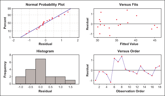
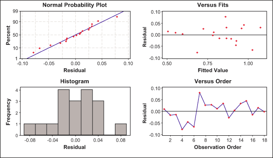
The residual plots of the difference between the fitted linear model and the experimental results are shown in Figures 7 and 8. These plots can be used as the goodness of fit for the models chosen. The normal probability plot and residuals versus fitted value plot shows that the residuals are close to the normal distribution and that there is no specific tendency.
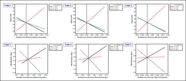
Next, practitioners analyze the influence of each component in relation to its responses at different amounts using Cox response trace plots (Figure 9). The trace plot shows how each component affects the response relative to the reference blend. In this example, the reference blend is the centroid of the design vertices. The total effect of a component depends on both the range of the component and the steepness of its response trace. The total effect is defined as the difference in the response between the effect direction point at which the component is at its upper bound and the effect direction point at which the component is at its lower bound.
Components with approximately horizontal response traces, with respect to the reference blend, have virtually no effect on the response, such as Monomer B for modulus (see red lines in the lower level of Figure 9). Components with similar response traces will have similar effects on the response, such as Monomer B and Monomer C for %H2O (see black and green lines in the upper side of Figure 9). Thus, the most influential variable to response modulus is Monomer C (see green line in the lower level of Figure 9).
Using similar analysis, practitioners can find that Monomer B is the most influential variable to %H2O. They can also see that the influence of variables on modulus does not always have the same direction as the influence of variables on %H2O. When the same component has responses with unparallel directions, it indicates that the mixture has a trade-off issue keeping it from reaching the optimal solution of its multiple responses.
Step 9: Find the Optimal Solutions of the Multiple Responses
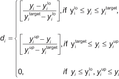
In many cases, multiple responses from a system have different magnitudes. In order to get fair “treatment,” responses with different magnitude must be normalized. The desirability function is a common method for multiple response problems. This approach scales the values of an individual response and its standard deviation to a desirability range between 0 and 1. Optimizing modulus and %H2O will help find the best nominal values of Modulus. A simple desirability function for nominal-the-best (NTB) targets is:
where:
yi represent values of individual response, i.e. modulus and %H20;
d is the related desirability function of y; and
ylo , yup and ytarget are the lower, upper and target values of the response.
Once responses are converted into individual desirability, weighted geometric mean aggregate methods may be used to combine the individual desirability using this formula:
Composite desirability = (d1w1 X d2w2) ^ 1/E2j=1wj
where:
w is weight.
Optimizing composite desirability is equivalent to optimizing the y responses.
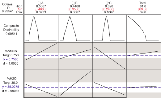
Given the range of modulus (0.75 ± 0.5 MPa) and the %H2O at ambient temperature (35 percent ± 3 percent), practitioners can find medical device ingredients with optimal desirable functions. One of the optimal mixtures is shown in Figure 10. The composite desirability of this mixture is close to 1. The optimal solution is at Total 1 percent, with the proportion of Monomer A, B and C at values 0.4088, 0.3506 and 0.2406, respectively. Thus, the optimal ingredients are Monomer A = (0.4088 x Total 1) percent, Monomer B = (0.3506 x Total 1) percent and Monomer C = (0.2406 x Total 1) percent. This result also indicates that practitioners could further pursue optimizing this total to an amount lower than Total 1 percent.
Replicating Procedure
This step-by-step process shows how to deal with mixture experiments found in many Six Sigma projects. This procedure can be used for any type of mixture experiment, including mixture of components only, mixture-factorial experiments and mixture-amount experiments.