Key Points
- p-Charts are a control chart used to see nonconforming data in a set of data.
- They can be used to pinpoint issues for further process improvement.
- Proper usage allows you to see the proportion of data falling outside of conformance.
Attribute control charts arise when items are compared with some standard and then are classified as to whether they meet the standard or not. The control chart is used to determine if the rate of nonconforming product is stable and detect when a deviation from stability has occurred.
The argument can be made that an LCL should not exist, since rates of nonconforming products outside the LCL are a good thing; we WANT low rates of nonconforming products. However, if we treat these LCL violations as simply another search for an assignable cause, we may learn from the drop in nonconformities rate and be able to permanently improve the process.
p-Charts can be used when the subgroups are not of equal size. The np chart is used in the more limited case of equal subgroups.
Why Use a p-Chart?
You’ll end up with quite a few data points throughout a project. As such, seeing where those points stack up is a handy way of optimizing your production. This is where the p-chart shines. By allowing you to see where points are exceeding the UCL or LCL, you can make adjustments as needed.
Steps in Constructing a p-Chart
- Determine the size of the subgroups needed. The size, n(i), has to be sufficiently large to have defects present in the subgroup most of the time. If we have some idea as to what the historical rate of nonconformance, p, is we can use the following formula to estimate the subgroup size:
n=3/p
- Determine the rate of nonconformities in each subgroup by using:
phat(i)=x(i)/n(i)
where:
phat(i)=the rate of nonconformities in subgroup i
x(i)=the number of nonconformities in subgroup i
n(i)= the size of subgroup i
- Find pbar; there are k subgroups.

- Estimate sigma-p if needed and determine the UCL and LCL:


- Plot the centerline, pbar, the LCL and UCL, and the process measurements, the phat’s.
- Interpret the data to determine if the process is in control.
Example:
Farnum Example:

data is from Farnum (1994):

Modern Statistical Quality Control and Improvement, p. 242

		Number

Day	Rejects	Tested	Proportion

1	14	286	0.0490

2	22	281	0.0783

3	9	310	0.0290

4	19	313	0.0607

5	21	293	0.0717

6	18	305	0.0590

7	16	322	0.0497

8	16	316	0.0506

9	21	293	0.0717

10	14	287	0.0488

11	15	307	0.0489

12	16	328	0.0488

13	21	296	0.0709

14	9	296	0.0304

15	25	317	0.0789

16	15	297	0.0505

17	14	283	0.0495

18	13	321	0.0405

19	10	317	0.0315

20	21	307	0.0684

21	19	317	0.0599

22	23	323	0.0712

23	15	304	0.0493

24	12	304	0.0395

25	19	324	0.0586

26	17	289	0.0588

27	15	299	0.0502

28	13	318	0.0409

29	19	313	0.0607

30	12	289	0.0415
Calculations:
PBAR = 0.0539
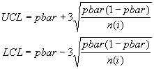
UCL = pbar + 3*sqrt(pbar*(1-pbar)/n(i))
LCL = pbar – 3*sqrt(pbar*(1-pbar)/n(i))
Day CL UCL LCL Proportion
1 0.0539 0.093892049 0.013808661 0.0490
2 0.0539 0.094246721 0.013453989 0.0783
3 0.0539 0.092310827 0.015389883 0.0290
4 0.0539 0.092126068 0.015574642 0.0607
5 0.0539 0.093410843 0.014289867 0.0717
6 0.0539 0.092624795 0.015075915 0.0590
7 0.0539 0.091587368 0.016113342 0.0497
8 0.0539 0.091943946 0.015756764 0.0506
9 0.0539 0.093410843 0.014289867 0.0717
10 0.0539 0.093822229 0.013878481 0.0488
11 0.0539 0.092498288 0.015202422 0.0489
12 0.0539 0.091240619 0.016460091 0.0488
13 0.0539 0.093209857 0.014490853 0.0709
14 0.0539 0.093209857 0.014490853 0.0304
15 0.0539 0.091883814 0.015816896 0.0789
16 0.0539 0.09314354 0.01455717 0.0505
17 0.0539 0.094103724 0.013596986 0.0495
18 0.0539 0.091646103 0.016054607 0.0405
19 0.0539 0.091883814 0.015816896 0.0315
20 0.0539 0.092498288 0.015202422 0.0684
21 0.0539 0.091883814 0.015816896 0.0599
22 0.0539 0.091528906 0.016171804 0.0712
23 0.0539 0.092688517 0.015012193 0.0493
24 0.0539 0.092688517 0.015012193 0.0395
25 0.0539 0.091470715 0.016229995 0.0586
26 0.0539 0.093683678 0.014017032 0.0588
27 0.0539 0.093011904 0.014688806 0.0502
28 0.0539 0.091823966 0.015876744 0.0409
29 0.0539 0.092126068 0.015574642 0.0607
30 0.0539 0.093683678 0.014017032 0.0415
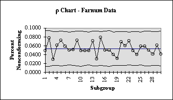
p – Chart:

Other Useful Tools and Concepts
Now that we’ve finished up with the calculations, you might be hungry for a little more. Having an out-of-control action plan is a handy way of keeping everything in check even when things go pear-shaped. Learning how OCAPs can impact your business is one of the most important steps in Six Sigma.
Additionally, you’ll be dealing with variations of all sorts when going through statistical analysis. Learning the differences between common cause and special cause variation is going to save a lot of time and energy on your part. You can learn all about it in our exhaustive guide.