The principles of Lean manufacturing are applicable to any business process. This article reviews some of the common problems seen in transactional projects and outlines an example where simple graphical methods are used to interpret cycle time data. Identifying and characterizing the non-Lean processes facilitates the application of 5S, brainstorming and other improvement tools with realistic goals for improvement.

When Lean principles are applied to transactional projects, data related problems might occur during the Measure and Analyse phases. Incomplete or non-normally distributed data, and data system confusion of cycle time and execution time definitions are typical issues that may arise. This article uses cycle time data to estimate process efficiency and average execution time and explores ways to statistically determine the vital Xs that drive inefficiencies in a process.

Process Capability and Gaussian Processes

Six Sigma involves a measure of process capability. The mean and standard deviation of the business process is combined with the upper and lower specification limits (USL, LSL) from the customer with the result reported in the form of defects per million opportunities (DPMO). The business process data usually results from the additive errors of a large number of random variations and follows the Gaussian or normal distribution (Figure 1). The areas falling outside of the customer specifications represent defects within the process.

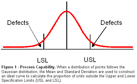
Gaussian distributions are commonly found in data generated by manufacturing processes. My experience is that very few transactional processes have the properties of a Gaussian distribution. By definition, transactional here means processes such as order entry, release of items from inventory or delivery to a customer site where the unit of measure is time. There is a groundswell of other practicing Six Sigma professionals that have also found the assumption of normality does not hold well in a transactional environment. In some cases, Black Belts will attempt to transform the data to force normality without considering the reason why the data has a non-normal probability distribution.

Lean Manufacturing – Time Is Money

Lean manufacturing, a process improvement discipline that evolved from solving manufacturing problems, concentrates on speed of execution. There is a large amount of data to support the business benefit of rapid execution. Internal metrics include the reduction of work in process (WIP) and a reduction in excess inventory, which restricts the use of capital and has a negative impact on cash flow. External metrics include faster time to market and increased customer satisfaction as work orders are completed more rapidly.

In a manufacturing environment, backlog and inventory build up physically and block workstations, floors and warehouse spaces. It is easy to see the clutter and appreciate the concept that WIP is tying up the company’s capital. Brainstorming sessions with the project team can proceed easily because the process owners have this physical, visual feedback of the vital X. This vital X becomes the little y for the Six Sigma project and the team starts to focus on the causes of the excess inventory and WIP. The business case is clear to everyone near to the project.

The reduction of clutter, the application of 5S and a visual workplace are effective improvement strategies in manufacturing environments. These strategies work well because they focus on the common causes of backlog, the common vital Xs for the little y, the WIP.

Calculating Lean Process Capability

In a typical manufacturing environment, processes are considered Lean when the efficiency of the process is 25 percent or more. Total time includes the setup, changeover, maintenance and scheduled downtime.

In a transactional environment, most of these measures have no counterpart. The equation is therefore modified to:

A transactional process is considered Lean when the execution time is less than one third of the delay time, or about 25 percent of the cycle time.

The Transactional Project Environment

When the focus of a project is to reduce cycle time, the idea is to reduce time required for the entire transaction. This concept may create difficulty for stakeholders involved in transactional projects because there is no physical, visible buildup of WIP. WIP levels in manufacturing are important because they represent the concrete, physical internal metric. The external metric, speed of execution, sometimes pales in comparison to the capital cost associated with WIP. In a transactional project speed to market and delivery time are the most important metrics. It is easier to lose focus because the metric is less visible in the transactional world. To achieve success, it is important to separate the individual cycle time data.

A typical business process is a succession of consecutive tasks (Figure 2). In many cases, the real time traps are found in the arrows joining the blocks. The arrows at the beginning and end of a sub-process are typically deemed out of scope during the Define stage. Rather than begin at the Xs with brainstorming and process mapping, it is better to start at the Y – the total cycle time for each step and break it into the separate components of execution time and delay time to facilitate identification of key drivers of variation.

Understanding Transactional Data

It is important for Black Belts to really understand the data that comes from their information systems. When pulling data from a typical data system, it is common to find that workers and IT systems are good at reporting when a task is completed, but not as good at reporting when a task began. People are anxious to get work off of their desk, not onto it. Even if start time data is available, workers worried about performance appraisals may manipulate it and rework does not usually get recorded. You will typically get data only at the signoff points. A common mistake made by Black Belts is to take the difference between signoff points thinking they represent execution times when in fact, this data represents cycle time. Direct measurements of separate delay and execution times are not captured.

A non-Lean process is more than 75 percent delay time and less than 25 percent execution time. Black Belts commonly try to reduce the cycle time by focusing on the execution process when the majority of the lost time is in the delay time. Delay times are usually related to management reviews, communication, handoffs, and roles and responsibilities that may slow the process.

Viewing individual events through a model allows observation of cycle time as a combination of an exponential distribution for delay time followed by a Weibull or Gaussian distribution for execution time. This is different from usual queuing theory assumptions, which are commonly modeled using two consecutive exponential distributions.

The following steps are presented to construct a delay step plus an execution step combination as a sample cycle. (Table 1 and Figure 3).

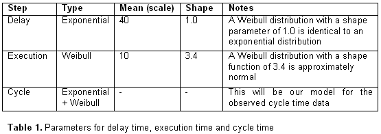
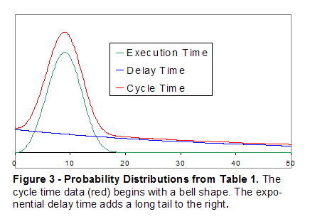
We can perform this analysis for a series of process steps and generate parameters for a more detailed analysis involving simulation to identify overall process bottlenecks.

A Real Transactional Process

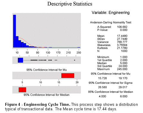
An example set of data was pulled from a transactional process improvement project at a heavy manufacturing company. For this project, each of the thirteen major steps from customer inquiry through quote generation, order conversion, fulfillment and final shipping were plotted in the same way to identify which steps produced the largest queues. This provided an estimate of a reasonable cycle time at each step. Bottlenecks were identified and examined to determine the causes for the largest delays.

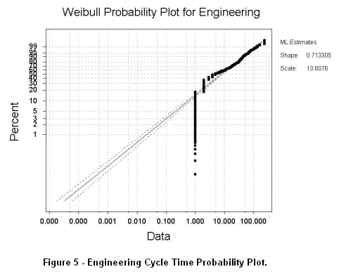
Figure 4 presents descriptive statistics associated with cycle time (in working days) for the engineering step of the extended process. The average cycle time is 17.44 days with a non-normal distribution skewed to the right. The probability plot is shown in Figure 5. From these data views we can estimate that about 20 percent of engineering requests are processed in one day, while 5 percent of the requests take longer than a month and a half. The delay time is the major portion of the cycle time. Further analysis of the data is a bit more complex, requiring math computations to calculate transactional process efficiency, but the basic principles are similar.

Calculation of Lean Metrics

The information we have so far is the Mean of the cycle time, an estimate of the proportion of steps that occur without delay (execution time) and the Mean execution time.

Starting from the individual subgroups, the overall average is calculated as:

since the total proportion must be 1:

substituting:

and rearranging

The efficiency of this process is about 5.7 percent – not very Lean. This is typical of transactional processes. The good news is that decreasing the delay time is usually much easier and cheaper than speeding up the execution time. Moving forward involves identification of the vital Xs that are driving the inefficiency of the process.

Hazard Plots

The Hazard plot shows the probability that something will occur given that it has survived to that time. Changes in the shape of the plot indicate whether the event is more or less likely to occur in the future. When combined with the probability plot, the Hazard plot provides additional information about the transition from one process to another. An example Hazard plot is shown in Figure 6.

A common feature seen with transactional cycle time data is that the exponential delay time shows up as a flat region on the hazard plot, extending out to very long times. The slope of near zero indicates that the probability of executing the job does not change with time. This is expected if the engineer puts jobs in his/her inbox and draws them out at random. It is important to point out that since the delay time is random, regression analysis will fail to show whether any Xs are influencing the length of delay.

The Hunt for Vital Xs – Binary Logistic Regression

Binary logistic regression is a valuable tool to use when the Y is discrete and the Xs are either discrete or continuous. The results are summarized in terms of the probability of the discrete event. Conclusions might take the following form: “The probability of closing the sale (discrete) increases by 83 percent for each hour (continuous) spent with the customer.” Or, “The probability of a delay occurring (discrete) increases by 75 percent if the order is international (discrete).”

When executing the Analyze phase of the example transactional manufacturing process, the cycle time for each step was examined to identify a clear end point for execution time and delay time. The individual jobs were classified as fast or slow for each of the process steps and a list of Xs was produced through brainstorming. Binary logistic regression produced a list of vital Xs for each step that affected whether the speed of the job at each process step. The project team then reviewed the list of vital Xs to determine an improvement strategy.

An example output from one of the regressions is reflected in Figure 7. The data shows that if the part is ordered less than three times a year it is significantly more likely to incur a delay.

Conclusion

This article presents some fairly simple tools for taking apart cycle time data, determining parameters of the underlying execution time and delay time and identifying the vital Xs that drive process efficiency. As a result, we know that:

• Execution time and delay time are not typically recorded in transactional systems.
• Hazard plots and probability plots are useful to separate cycle time data into components of execution time and delay time.
• Realistic targets for cycle time are derived from the same plots.
• A continuous variable (time) is used to flag jobs as discrete events (fast/slow).
• Binary logistic regression is helpful to determine the list of vital Xs to focus improvement efforts in Lean Six Sigma projects.

These tools will provide insight into the amount of delay time in a process and assist in setting realistic targets for execution time. In addition, statistical verification of the vital Xs influencing delay time will help direct the project improvement focus through the application of the Lean toolkit (e.g., 5S, visual workplace, roles and responsibilities, handoff management, communication plan, etc.)