When working with data sets, practitioners sometimes encounter metrics, such as out-of-roundness and loss-of-moisture measurements, with physical limits. In these scenarios, the data distribution is truncated at the value of physical limitation, creating a distribution outside of the criteria of a normally distributed population. With non-normal data, estimates and predictions using the normal distribution are not accurate, creating the need for alternative methods of analysis to assess the data.

Standard Methods

Typically, when data does not fit the normal distribution and prediction or estimation calculations are made using the assumption of normality, data is transformed and assessed for normality. If the transformed data fits the normal distribution, then calculations are performed using the transformed data with transformed specification limits. Alternatively, if other distributions are found that fit the non-normal data, the capability of the process can be calculated using an alternative distribution, which better fits the data. However, if no alternative distribution is found that fits the data and the data cannot be transformed into a normally distributed data set, other methods of analysis are necessary.

Alternative Method

Due to the nature of truncated data sets, which have a point of central tendency at a physical limit, common transformation methods such as Box–Cox and Johnson are often not sufficient. The following method of estimating the population’s standard deviation for the normal distribution is a practical method that gives a realistic estimate of the standard deviation. It also avoids violation of the assumption of normality when using the C_pk calculation based on the normal distribution. This correction provides practitioners with the ability to predict the spread of the data and assess capability in the direction of the upper specification limit. Prior to using this correction method, however, practitioners must verify that the sample data is of adequate size to approximate the normal distribution.

Empirical research and data results, gathered from both theoretical and production data and analysis, support the theory that estimating the standard deviation is possible for physically limited data by proceeding as if the data were not truncated. Theoretically, this means extending the data beyond the physical limitation of the measurement.

The empirical evidence provides a ratio, or correction factor, between the truncated distribution standard deviation and the theoretical normal distribution. The equation is:

where

is the standard deviation calculated from the physically limited data set truncating one side of the data.

is the standard deviation calculated for the population if the data were not truncated.

The coefficient of 1.7 correlates these two parameters.

This ratio can act as a correction factor for the standard deviation, allowing practitioners to calculate the C_pk based on the assumption of normal data. An accurate calculation of process capability or any other estimate or prediction made using the normal distribution is not valid without this type of correction. In the following example, the standard deviation is estimated for the population using the correction factor.

Example Data Description

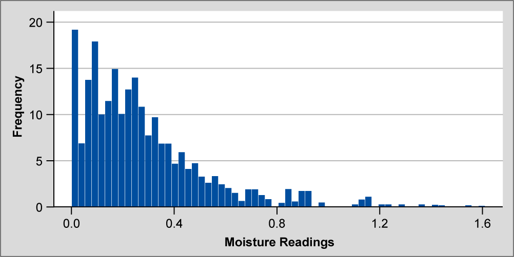
In the figure below, the distribution is truncated as it approaches approximately zero readings of moisture. This truncation is due to the physical limitation of the zero bound on a moisture reading (i.e., a product cannot have less than zero units of moisture present). Hence, the data is not able to follow the normal distribution.

This truncation can cause the central tendency measurement to match the physical limit value if that is desirable. With out-of-roundness and loss-of-moisture measurements, often there is only an upper specification limit and it is desirable to have low values, as is the case with the data in Figure 1.

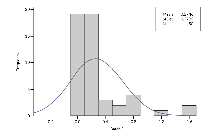
The standard deviation for this example data set is 0.3735 units. The estimated (or corrected) standard deviation for the example data set as a normally distributed data set is 0.3735 units multiplied by 1.7, which is equal to 0.6350 units. The mean from the example data set is 0.2746 units. The specification limit is a one-sided upper specification limit (USL) of 8 units.

The following equation is typically used to calculate process capability:

, where

USL and LSL are upper and lower specification limits

is the population standard deviation

is the population mean

However, because no LSL exists in this case, the equation is reduced to:

This alternative process capability estimation can be used for further analysis.