Those in the information technology (IT) field often encounter service level agreements (SLAs) that define the performance a customer can expect from a particular process or service, such as a help desk. Often, these agreements are established by negotiation rather than by a more scientific approach that would be used in a Six Sigma process (where SLAs would more often be known as specification limits).

There is an approach for setting SLAs that can help avoid most common mistakes. It can be applied in many situations without making a commitment to full-blown Six Sigma training and deployment. The simplified illustration included here does not assume the reader is statistically trained and it is configured with a smaller set of data than would be expected in actual practice. In the interest of simplicity and clarity, certain technicalities and qualifications which may apply in rare circumstances are not addressed.

Basic Terminology and Concepts

Every process exhibits variability – sometimes things get done quickly, and sometimes they do not. The time it takes to drive to work, response time to display a web page, the length of the teller line at the bank are all everyday things that are variable. Understanding that variability is essential to establishing SLAs that are meaningful to the customer and achievable by the provider.

The amount of variability inherent in a process can be measured by the “standard deviation” (if the elements of data are “normal” – an issue to be examined later). There is no need to go into the underlying math to understand the concept and power of this measure. At its most basic level, standard deviation is simply a value that tells how much of the variation is contained within a certain range of process performance, as specifically enumerated in the table.

Three standard deviations (also called 3 sigma) means that less than 3 outcomes per thousand opportunities, or executions of the process, are expected (statistically speaking) to be outside the numerical range defined by +/- 3 sigma. Here is what this means in a particular process:

Assume a business is running an IT help desk, and the business has a set of historical data on how many days it takes to close cases. The business wants to establish an SLA for days-to-close cases with its customer. To get a first approximation, the business might use a basic tool such as “descriptive statistics” to find the range of values in its data set – the average or mean, and the standard deviation.

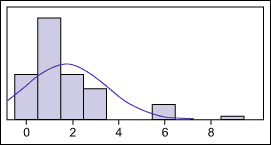
In the particular data set being used, the minimum value is zero days, the maximum is nine days, the average is 1.69 days and the standard deviation is 1.74 days. With one important qualification (to be addressed in a moment), this information tells us that 68.26 percent of the time a case will be closed in not more than 3.4 days (1.69 + 1.74). Similarly, 99.73 percent of the time a case will close within 6.9 days (1.69 + 3 * 1.74). So, at first glance, the business might be inclined to set its SLA to guarantee 99.7 percent of cases will close within 6.9 days.

The qualification: The foregoing logic gives correct results only if the data is normally distributed – that is, when the data is charted its produces the well-known bell-shaped curve, with about half of the data points above and below the mean.

Looking for Normally Distributed DataWhen looking at the data in Figure 1, it is clear that that this condition is not satisfied. The data is “skewed” so that there is a long “tail” to the right. The visual impression is confirmed by a statistical test (the Anderson-Darling Normality Test, not shown) that indicates there is less than a .5 percent chance that this data is, in fact, normal.

Figure 1

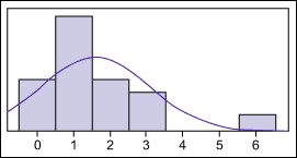
From visual examination it can be seen that there is one data point at about 9 days. This is a lot different than any of the other data, so the business must wonder why. This sort of data, commonly called an “outlier,” is probably the result of what is known as an assignable cause.Upon investigation, the business finds that the case was actually completed in two days, but was not closed because the system only allows a case to be closed by the person to whom it was assigned. In this instance, that person was out sick for a week, so the case did not close until they returned.The business corrects the data and then takes another look at the overall distribution – Figure 2. It is still not normal. There seem to be two peaks in the data – one at about 1 day and another about 6 days. This pattern is known as a bimodal distribution, and is often an indication that the data actually represents more than one process, rather than the single process the business may have initially assumed.

Figure 2

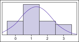
When investigating this bimodal pattern by taking a careful look at the subset of the data that took 6 days to close, the business discovers that all of the cases relate to data corruption problems, which are not handled by the help desk. Cases of this type are handed off to the data management group and are dealt with by a process that is very different from other calls. Hence, the businesses decides to exclude these from the data set it is using to set the SLA for all other types of calls. This gives the business the data set shown in Figure 3.While, strictly speaking, this data is still not normal, the range and distribution are now quite tight and the business can use standard deviation to set its SLA without risk of forming wrong conclusions.Creating Reasonable SLAsConsequently, the business proposes to set the SLA for days-to-close cases not related to data corruption at 2.3 days (1.3 mean + .96 std.dev.). That is far different than the initial impression of 4.3 days.In this example, the business will end up creating two different SLAs – one for data corruption cases as well as one for other types.This simple approach can be applied to many types of historical data. It will lead to SLAs that are more meaningful and useful than those produced by negotiation.