Manufacturing facilities can be faced with major challenges when it comes to process improvement, largely because practitioners don’t always know enough about the underlying process factors (x’s) are that drive the improvement metric (Y).
Practitioners might have a brainstorming session to tap into the collective experience of experts involved in the process, and design experiments to first uncover and then assess the importance of likely variables. Afterward, following rounds of experimental work that may generate thousands of pounds of off-grade material, these factors might be identified, and the process optimized around them.
This process may have generated a history of product performance together with associated process data – sometimes hundreds of x’s, each with thousands of data points. Yet the task is just too cumbersome; the relationships are often too complex to search randomly for relationships between Y and various combinations of the x’s. Recursive partitioning, a data-mining strategy commonly used in the medical field, can cut through the clutter, frequently providing the line engineer with the crucial relationship he or she is looking for in a shorter time than is needed for a traditional design of experiments.
Optimizing a Process’ Categorical Response
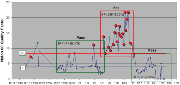
Before I describe this data mining strategy, consider these two examples drawn from the chemical industry. A nylon quality factor – a pass/fail metric – is tracked in Figure 1 as it drifted through periods of good and bad performance (in this figure, P indicates the quality factor was below the control limit, while F means the factor was above the control limit). This polymer manufacturing process routinely generated readings for 600 x’s – things like rates, temperatures and pressures. The line engineer needed to identify those x’s responsible for driving the quality factor.
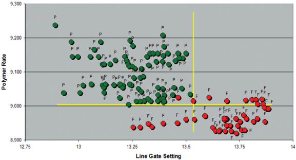
Data from 126 production lots was collected for each x, then a recursive partitioning strategy was used to identify, in this case, the two factors most important to driving the quality factor from the 600 variables being monitored. Run charts for these two are shown in Figure 2. The P’s and F’s over the line gate data indicate the pass/fail metric for the quality factor at that point in time. Generally, as the polymer rate went down and/or the line gate setting moved higher, the polymer quality factor failed.
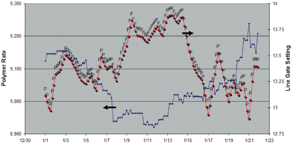
Figure 3 contrasts these two process factors driving the nylon’s quality factor. Again, the P’s and F’s designate the pass/fail regions of Figure 1. Now, it’s obvious where this process should run with respect to these two variables. No experiments were run; instead, a quick analysis of the process data history turned up an answer that could explain 89 percent of the quality factor’s variance over this time period. This example demonstrates how historic process data can be used to explain a binomial pass/fail response. I call this data-mining approach “matching process variables to a categorical Y-mask” (here, the P and F grades).
Optimizing a Process’ Continuous Response
The second example treats continuous data: The iron (Fe) concentration in a process stream that is measured monthly over a 36-month period; ten process variables were measured as well. The questions were: Which of these variables tracked iron concentration and what was their explicit relationship?
A recursive partitioning strategy identified two process factors (x factors 1 and 2) that are influential to iron levels. Together, they explained 74 percent of the iron data’s variation. Once the recursive partitioning strategy identified the important x’s, the next step was to code each x to its respective Z score (subtract each x data mean and divide by its standard deviation), then use conventional multilinear least squares analysis to determine the second-order model’s parameters:
Expression 1: Y = b0 + b1x1 + b2x2 + b12x1x2 + b11x12 + b22x22
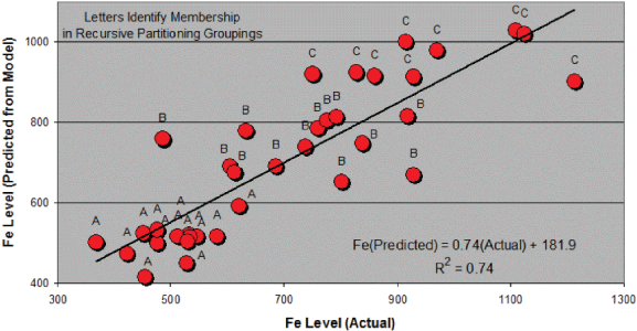
A standard regression treatment led to the following model with R2 = 0.74 (the model explained 74 percent of the variability in the iron data):
Expression 2: Fe (predicted) = 737 + 46.3x1 – 143.9x12 + 204.1x2 + 188.0 x1x2
More generally, the second-order model with n x’s will require an intercept (bo), n main effects (b1 to bN), n square effects (b11 to bNN) and (n/2) x (n-1) 2-factor interactions (b12 to b(N-1)bN). Only those judged to be significant in the regression will be kept in the final expression.
Figure 4 tracks the two process factors – the actual iron concentration and the iron concentration predicted from Equation 2. Letters A, B and C denote unique group membership that was created by partitioning the iron data twice in a recursive partitioning treatment. Over this 36-month period, iron concentration rose as either process factor increased.
Note, when building a model like Equation 1, all x data (not Y data) needs to be coded to its respective Z scores for two reasons: 1) for uncoded data, square terms are likely to be collinear (functions of) their main effect and 2) differences in magnitudes for the various x’s can cause rounding errors in the matrix multiplication used by regression programs.
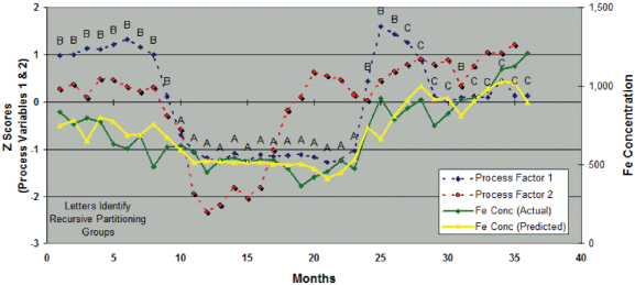
Figure 5 draws the relationship between actual and predicted iron levels over this 36-month period. The partitioned groups concentrated the A group at low levels, the C group at high levels and the B group at intermediate levels. Low iron concentrations would be expected by the process operating under group A conditions (each defined by a specific range of x1 and x2).
Generally, practitioners can use the recursive partitioning strategy to identify specific process x’s – from the many that are being collected – that drive a process Y. If the Y is categorical, as demonstrated in the first example, a categorical Y-mask can be created against which the x’s can be matched and process charts, like Figure 3, can be drawn. When the Y data is continuous, however, as demonstrated in the second example, those few x’s that provide the best fit to Y can be identified, and then the explicit relationship between the Y and x’s (like Expression 2) can be determined through standard regression techniques (e.g., 36 Y’s were regressed against 36 x1 and x2 pairs in a full second-order model that was reduced to contain only significant parameters.
Partitioning Variance
Any group of numbers can be described by their average and variance. If nothing else is known about their underlying population, the best model for this group is just that: the average and variance. Models, however, can be developed to explain a portion of the variance, and the degree to which a model explains a variation is quantified through an analysis of its total sum-of-squares (TSS in Expression 3, where n equals the number of data points). The more the model explains, the better the fit.
Expression 3 results from rearranging of the standard variance expression, and R-square is the percentage of TSS explained by the model, be it a regression expression or a simple factor analysis, where different segments of data have been grouped (e.g., 74 percent of TSS was explained by the iron concentration model described in Expression 2).
Expression 3: ![]()
If a practitioner knows something further about the set of numbers – such as the fact that different machines were involved or different shifts or different feed stock – they can factor that variation component from the TSS as known. These known differences account for a portion of the overall TSS.
Expression 4 segregates subsets of the numbers into two or more subgroups (recursive partitioning segregates only two). The single summation breaks into double summations (partitioning n data into their m1 and m2 subgroups), and adds and subtracts group means within the parenthesis for zero effect inside the parenthesis. Expression 4, thus, is identical to Expression 3; it’s simply using more information.
Expression 4: ![]()
Expression 5 (not shown) groups terms in the expression, but again nothing’s changed. When the squared multiplication is carried out, two square terms result, (Expression 7), because the interaction term ( Expression 6) sums to zero, as this summation is being taken across all deviations, not their squares.
Expression 6: ![]()
The right side of Expression 7 is that portion of TSS that’s been explained by grouping the Y data into two subgroups. The left-side summation is what’s left of TSS that is unexplained (the variation within each group).
Note: if the model does not explain Y’s variation very well, the group means become nearly equivalent, and Expression 7 reduces back to Expression 3. The overall mean remains the best model for the data.
Expression 7: ![]()
“within” & “between” groups
Expression 7 simplifies to Expression 8, where m is the number of members in each group.
Expression 8: ![]()
TSS can now be reduced by that amount of the variance explained by the model to TSS’ as shown in Expression 9.
Expression 9: ![]()
“Explained” “Unexplained”
Recursive Partitioning Strategy
A recursive partitioning strategy systematically takes each column of x data (often as many as 600 x’s), sorts each x and Y, and then systematically partitions the sorted Y data into two subgroups, starting with smallest Y value in subgroup 1 and the rest of the Y values in subgroup 2. The splitting operation proceeds in steps by systematically transferring the smallest value from subgroup 2 to subgroup 1. At each step the percent of TSS explained by that partition is calculated utilizing Expression 8. The ideal split of Y for that x is the one producing the largest R2. Thus, this x-induced split of Y will lead to a reduced TSS (i.e., some of the original TSS will have been explained).
To this point, Y data will have been split into two subgroups based on the fit to the most important x. Each of Y’s subgroups can then be subjected to the same strategy for the string of x’s to find the next best x and its best split. This strategy becomes clearer with the following example (Table 1), where 10 Y values have been systematically split against 10 x1 values (upper right part of Table 1).
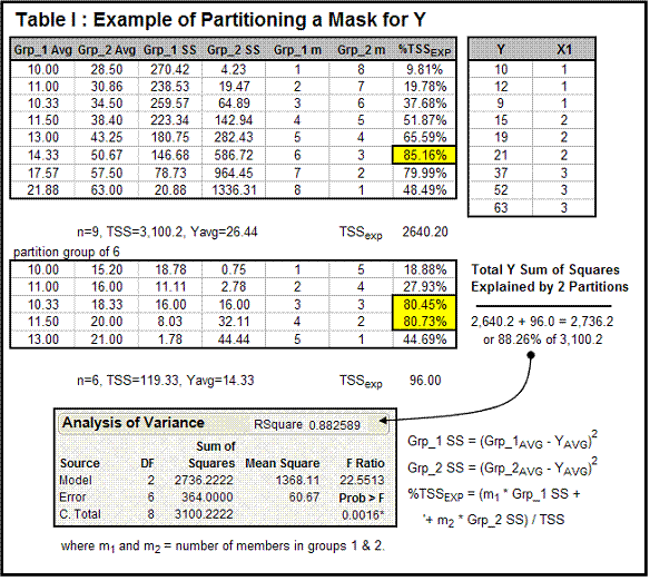
Table 1 tracks the partitioning possible for nine data points, where three machines constitute a categorical variable x1: Y’s average is 26.44 and its TSS is 3,100.2. The question becomes: Are we able to explain a significant portion of Y’s TSS by partitioning the nine data points into multiple groups? That is equivalent to asking whether Y shows any dependence on x, the machine mask.
Each row of the table tracks the results of a specific split. For example, the first split of Y would have the first Y value of 10 in Group 1 and the remaining nine (12, 9, … 63) in Group 2. Each group average, its “within sum of squares” (from Expression 7) and the number (m) of members of each group are used to calculate the percentage of variance explained by that split (%TSSEXP). In this case, the split of six in Group 1 and three in Group 2 explained the greatest proportion of Y’s variation: 85.2 percent of the total variation. Note, appropriate formulas are depicted in the lower right portion of the table.
Each subgroup can now be taken separately through this partitioning strategy to look for further associations – hence, the strategy’s name, recursive partitioning. The lower part of the table tracks further partitioning of Group 1.
Note: the total variation explained in the two splits (88.26 percent of Y’s 3,100.2 variation) was equivalent to the R2 one would obtain in a typical ANOVA (analysis of variance) calculation. Of course, if there were hundreds of x’s to choose from, the ANOVA would be tougher to decipher.
This is a trivial example utilizing masked data. In the real manufacturing world, there might be a thousand x’s to choose from, each with a thousand data points. This adds up to 1 million data points to sort through – the proverbial needle in a haystack.
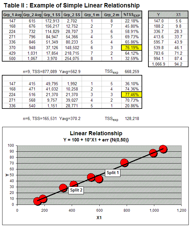
The second example (Table 2) is a continuous one, where Y is a linear function of x. Note that “err{N(0,50)}” is an error term meaning “normally distributed with mean zero and standard deviation 50.” Here, the greatest percentage of TSS is explained by Y partitioning based on the six smallest x1 values and the other three (split 1 on the chart). Another 77.46 percent of that group’s variation could be explained by splitting the six into two groups of three. Thus, the partitioning strategy would have chosen x1 (from potentially hundreds of x’s not shown) to then regress Y against to develop the final model shown at the bottom of the table.
Again, both examples are trivial and meant to show how the recursive partitioning strategy works. For a real process, there would be many more x’s, and this strategy would be used to pick out those best fitting the Y.
In this same manner, more complicated relationships involving several x’s could be identified and then these used to build an explicit model (like that in Expression 1) through standard regression techniques.
Note: The author’s Excel program PARTITION (available on request) can be used to perform recursive partitioning and was used to generate the models developed in this work.
