Everyone is taught in school the equation of a straight line:

Y = a + bX

Where a is the Y-intercept and b is the slope of the line. Using this equation and given any value of X, anyone can compute the corresponding Y.

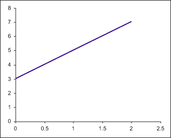
In Figure 1, Y = 3 + 2X. It is easy to see visually that a is 3. For the slope b, any two points on the line need to be chosen, say X1 = 1, Y1 = 5 and X1 = 2, Y1 = 7 and apply the following formula:

Method of Least Squares

Now suppose in real life the following data points are collected:

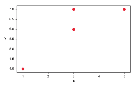
How can one figure out the equation of the line that is drawn through the middle of these set of points? Statistically, the best fitted line is the one that minimizes the error between the points on the line (also called the fits or Y-hat) and the actually observed data points.

The easiest way to determine this line would be to calculate the sum of the differences between the fits (Y-hat) and the actual observed points (Y). But this method sometimes does not work because the positive and negative values may cancel each other out to obtain zero. A better method is to obtain the sum of the absolute difference. But this method does not stress the magnitude of the error.

However, if one squares the difference before they are added, two things are achieved:

1. It cancels the effect of having both positive and negative values
2. It magnifies (penalizes) the larger errors

Hence, one would choose the model with the least squares difference. But how can anyone tell if they have in fact found the best fitting line? Is there another line that will give an even lower least squares difference?

Statisticians have found that the line with the best fit has the following slope:

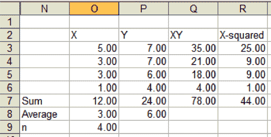
To find a:

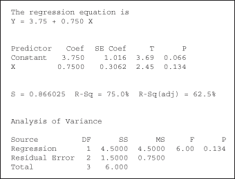
Hence, Y-hat = 3.75 + 0.75X is the best fitted line.

Standard Error of Estimate

Intuitively it is clear that a line is a better estimator of the data points when the points lie close to the line, than when they lie far away from the line. One needs a way to measure the scatter of the observed values around the regression line. This can be done via the standard error of the estimate:

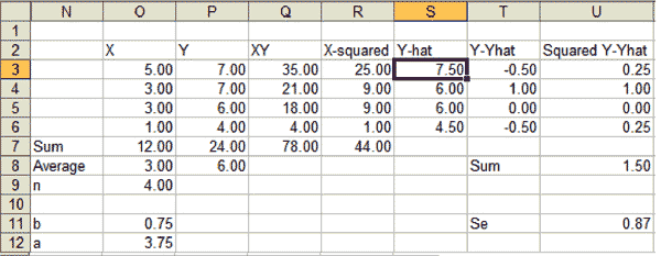
The larger the Se, the larger the dispersion of the points around the regression line. In the Minitab output, this is given by the s symbol. Assuming the points are normally distributed around the regression line, one would expect 68 percent of the points within ± 1Se, 95.5 percent within ± 2Se and 99.7 percent within ± 3Se.

Coefficient of Determination and Coefficient of Correlation

One also can obtain the coefficient of determination, or R² or R-Sq(uared). This is:

And the coefficient of correlation or r is:

R-squared provides the percentage of variation in Y that is explained by the regression line:

Figure 3 shows the Minitab output of the same case showing the regression line, Se and R-Sq.

Significance of the Model: The F Statistics

A 75 percent explained variation sounds pretty good. This model seems to be a representation of the data points. But is this really true? There are only have four data points – almost every line would look good if there were only a few data points? Therefore a much more important indicator of the validity of the model is – as always – the p-value.

The p-value in a simple linear regression is determined via the so-called F statistics: An F-value is calculated as the quotient of the variation that is caused and can be explained by the X in the model (in Minitab: mean of sum of squares for regression [MS regression]) divided by the variation that is caused by other variables which are not included in the regression, the error (in Minitab: mean of sum of squares for regression [MS residual error]). Logically, the more variation can be explained by the X and the less is unexplained the higher the F-value. In this case, F = 6. But is this already high enough to conclude that the variation explained by the X is significantly higher than the unexplained variation?

In order to retrieve the p-value, one now uses the F-tables (easiest is to use is Excel’s FDIST function), for DF regression = 1 and DF error = 2. DF regression is 1 because there is only one X in this case. And since total DF as usual is n-1 (i.e., 3) DF error is 2 (= DF total – DF regression)

In this case, the p-value is 0.134. If alpha is set at 0.05, then one would have to reject this regression line as having a valid fit because p-value is greater than 0.05. This means that the model is not significant. The R-Sq value – though looking quite good –is of no value and should not be interpreted. Those who did this regression will need to collect more data, re-do the regression and then see whether the p-value is now significant before they interpret the R-Sq value.