
What is non-normal data? Normally distributed data is a commonly misunderstood concept in Six Sigma. Some people believe all data collected and used for analysis must be distributed normally. But normal distribution does not happen as often as people think, and it is not a main objective. Normal distribution is a means to an end, not the end itself.
Defining Non-normal Data
Normally distributed data is needed to use several statistical tools, such as individual control charts, Cp/Cpk analysis, t-tests, and the analysis of variance (ANOVA). If a practitioner is not using such a specific tool, however, it is not important whether data is distributed normally. The distribution becomes an issue only when practitioners reach a point in a project where they want to use a statistical tool that requires normally distributed data and they do not have it.
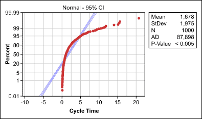
The probability plot in Figure 1 is an example of this type of scenario. In this case, normality clearly cannot be assumed; the p-value is less than 0.05 and more than 5 percent of the data points are outside the 95 percent confidence interval.
What can be done? There are two options:
- Identify and, if possible, address reasons for non-normality or
- Use tools that do not require normality
Addressing Reasons for Non-normal Data
When data is not normally distributed, the cause for non-normality should be determined and appropriate remedial actions should be taken. Six reasons are frequently to blame for non-normality.
Reason 1: Extreme Values
Too many extreme values in a data set will result in a skewed distribution. The normality of data can be achieved by cleaning the data. This involves determining measurement errors, data-entry errors, and outliers, and removing them from the data for valid reasons.
Outliers must be identified as truly special causes before they are eliminated. Never forget: The nature of normally distributed data is that a small percentage of extreme values can be expected; not every outlier is caused by a special reason. Extreme values should only be explained and removed from the data if there are more of them than expected under normal conditions.
Reason 2: Overlap of Two or More Processes
Data may not be normally distributed because it comes from more than one process, operator or shift, or from a process that frequently shifts. If two or more data sets that would be normally distributed on their own are overlapped, data may look bimodal or multimodal – it will have two or more most-frequent values.
The remedial action for these situations is to determine which X’s cause bimodal or multimodal distribution and then stratify the data. The data should be checked again for normality and afterward, the stratified processes can be worked with separately.
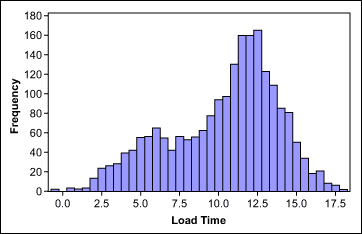
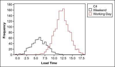
An example: The histogram in Figure 2 shows a website’s non-normally distributed load times. After stratifying the load times by weekend versus working day data (Figure 3), both groups are normally distributed.
Reason 3: Insufficient Data Discrimination
Round-off errors or measurement devices with poor resolution can make truly continuous and normally distributed data look discrete and not normal. Insufficient data discrimination – and therefore an insufficient number of different values – can be overcome by using more accurate measurement systems or by collecting more data.
Reason 4: Sorted Data
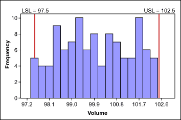
Collected data might not be normally distributed if it represents simply a subset of the total output a process produced. This can happen if data is collected and analyzed after sorting. The data in Figure 4 resulted from a process where the target was to produce bottles with a volume of 100 ml. The lower and upper specifications were 97.5 ml and 102.5 ml. Because all bottles outside of the specifications were already removed from the process, the data is not normally distributed – even if the original data would have been.
Reason 5: Values Close to Zero or a Natural Limit
If a process has many values close to zero or a natural limit, the data distribution will skew to the right or left. In this case, a transformation, such as the Box-Cox power transformation, may help make data normal. In this method, all data is raised, or transformed, to a certain exponent, indicated by a Lambda value. When comparing transformed data, everything under comparison must be transformed in the same way.
The figures below illustrate an example of this concept. As illustrated, figure 5 shows a set of cycle-time data; Figure 6 shows the same data transformed with the natural logarithm.
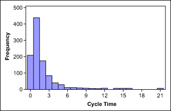
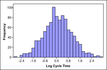
Take note: None of the transformation methods provide a guarantee of a normal distribution. Always check with a probability plot to determine whether the normal distribution can be assumed after transformation.
Reason 6: Data Follows a Different Distribution
Many data types follow a non-normal distribution by nature. Examples include:
- Weibull distribution, found with life data such as survival times of a product
- Log-normal distribution, found with length data such as heights
- Largest-extreme-value distribution, found with data such as the longest downtime each day
- Exponential distribution, found with growth data such as bacterial growth
- Poisson distribution, found with rare events such as number of accidents
- Binomial distribution, found with “proportion” data such as percent defectives
If data follows one of these different distributions, it must be dealt with using the same tools as with data that cannot be “made” normal.
No Normality Required
Some statistical tools do not require normally distributed data. To help practitioners understand when and how these tools can be used, the table below shows a comparison of tools that do not require normal distribution with their normal distribution equivalents.
| Comparison of Statistical Analysis Tools for Normally and Non-Normally Distributed Data | ||
| Tools for Normally Distributed Data | Equivalent Tools for Non-Normally Distributed Data | Distribution Required |
| T-test | Mann-Whitney test; Mood’s median test; Kruskal-Wallis test | Any |
| ANOVA | Mood’s median test; Kruskal-Wallis test | Any |
| Paired t-test | One-sample sign test | Any |
| F-test; Bartlett’s test | Levene’s test | Any |
| Individuals control chart | Run Chart | Any |
| Cp/Cpk analysis | Cp/Cpk analysis | Weibull; log-normal; largest extreme value; Poisson; exponential; binomial |
Other Useful Tools and Concepts
Now, we’ve discussed non-normal data at length. but there are tools to account for unforeseen circumstances. Force field analysis is one such tool, weighing the factors that can drive or deter a change in your processes. Mastering how to create one of these documents can prevent headaches later on.
Further, it is worth exploring the role the x-bar plays in your statistical analysis. This is a basic concept, but one that most analysis hinges upon. As such, learning how to calculate and apply it to your analysis should be one of your first steps if you’re new to statistics.
Conclusion
Hopefully, you come away from this guide armed and ready to deal with non-normal data. Just like normal data, you have a variety of tools capable of dealing with the situation. Remember, learning these methods isn’t an overnight thing, so make sure to apply the principles as needed until they stick.