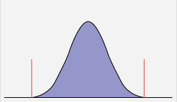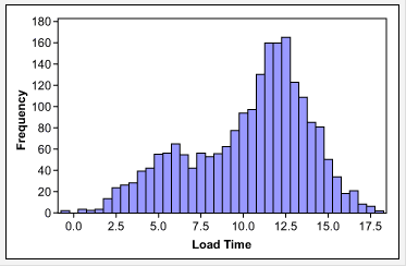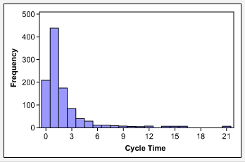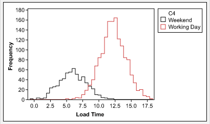
The distribution of data can be categorized in two ways: normal and non-normal. If data is normally distributed, it can be expected to follow a certain pattern in which the data tend to be around a central value with no bias left or right (Figure 1). Non-normal data, on the other hand, does not tend toward a central value. It can be skewed left or right or follow no particular pattern.

Non-normal data sounds more dire than it may be. The distribution becomes an issue only when practitioners reach a point in a project where they want to use a statistical tool that requires normally distributed data and they do not have it.
Non-normality is the result of either:
- Data that contains “pollution,” such as outliers, the overlap of two or more processes (Figure 2), the result of inaccurate measures, etc.
- Data that follows an alternative distribution, such as cycle time data, which has a natural limit of zero (Figure 3).


To move forward with analysis, the cause of the non-normality should be identified and addressed. For example, in the case of the website load time data in Figure 2, once the data was stratified by weekends versus working days, the result was two sets of normally distributed data (Figure 4). Each set of data can then be analyzed using statistical tools for normal data.

If the data follows an alternative distribution (see table below for common non-normal distribution types), transforming the data will allow practitioners to still take advantage of the statistical analysis options that are available to normal data. The best method for transforming non-normal data depends upon the particular situation, and it is unfortunately not always clear which method will work best. A common transformation technique is the Box-Cox.
| Common Non-normal Distribution Types | ||
| Distribution | Type Data | Examples |
| Lognormal | Continuous | Cycle or lead time data |
| Weibull | Continuous | Mean time-to-failure data, time to repair and material strength |
| Exponential | Continuous | Constant failure rate conditions of products |
| Poisson | Discrete | Number of events in a specific time period (defect counts per interval such as arrivals, failures or defects) |
| Binomial | Discrete | Proportion or number of defectives |
Another option is to use tools that do not require normally distributed data. Testing for statistical significance can be done with nonparametric tests such as the Mann-Whitney test, Mood’s median test and the Kruskal-Wallis test.
To learn more about non-normal data and related topics, refer to the following articles and discussions on iSixSigma.com:
- Are You Sure Your Data Is Normal?
- Dealing with Non-normal Data: Strategies and Tools
- Non-normal Data Needs Alternate Control Chart Approach
- Process Capability Calculations with Non-Normal Data
- Tips for Recognizing and Transforming Non-normal Data
- Making Data Normal Using Box-Cox Power Transformation
- Trying to Make Sense of Non-normal Data
- Non-normal Data: Transform?
- Non-normal Data: Use Control Charts?
- Non-normal Data on Control Charts – Transformation Versus Percentile Methods
- Non-parametric Data – Which Factor Has the Greatest Influence?
- The Cox-Box: Data Transformation
Non-normal data is a typical subject in Green Belt training. To learn more about non-normal data and hypothesis testing, purchase the Six Sigma Green Belt Training Course available at the iSixSigma Store.