This article is the last of four parts. It presents a discussion of opportunities for defects (OFD), defects per million opportunities (DPMO) and Sigma levels. When comparing implementations across companies, using the common language of DPMO and Sigma levels will assist in understanding benchmarking data. Parts one, two and three followed a progression of goals shared by both software development and Six Sigma: 1) Reducing released defects; 2) Finding and fixing defects closer to their point of origin; 3) Predicting and tracking defect appearance and removal rates and repair costs; 4) Comparing implementations within the company; 5) Comparing implementations across companies.

The Poisson Model

Some key Six Sigma concepts and terms are built on the Poisson distribution, a math model representing the way discrete events (like defects) are sprinkled throughout physical, logical, or temporal space. Sparse defects typically follow a Poisson distribution, making the model’s mapping of defect probability a useful tool. The model predicts the probability of finding zero defects in a unit (or the proportion of a series of units) is e-DPU, sometimes called first time yield (FTY). In our example (Equation 1) where DPU = 1, the FTY = about 36.8 percent. This example will serve as a backdrop for studying the influence of the area of opportunity within a unit.

Area of Opportunity

The Poisson distribution provides a sense of the area of opportunity for the events or defects it tracks. When DPU = 1, some units (about 36.8 percent per Equation 1) are expected to contain zero defects.

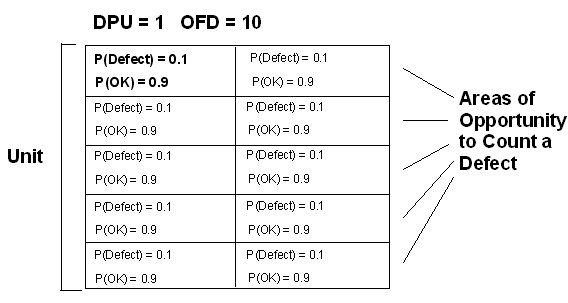
Let’s picture the example unit as containing 10 areas of opportunity, each representing a region where a single defect either will or will not be found (Figure 1). For the overall defect per unit (DPU) to reach 1, each of these 10 opportunities for defect (OFD) regions must actually contain a defect only 1 time in 10 (p(defect) = 0.1). In other words, the chances that any single OFD is defect free (OK) must be 9 in 10 (p(OK) = 0.9).

For the unit to be defect free, all 10 OFDs must be defect free. The concept of joint probability provides that the chances of all 10 independent OFDs being defect free is the product of the probabilities for each one being defect-free. Equation 2 shows that this equates to about 34.9 percent. It is no accident that this agrees pretty well with the estimate in Equation 1 (36.8 percent), as the Poisson distribution is built on the basis of simple probability related to individual discrete events.

The Poisson FTY estimate will track with the OFD estimate (Equation 2) regardless of the exact number of opportunities. For example, if the OFD count in the example unit where DPU = 1 is not 10 but 100, the chances of each OFD containing a defect is 1/100. The chance of each OFD being defect free is 99/100, creating a defect free unit probability of 0.99100 or about 36.6 percent – closer still to the Poisson estimate (36.8 percent).

Defects Per Million Opportunities (DPMO)

A meaningful comparison of defect counts for different work products requires some normalization for size. Defects per million opportunities (DPMO) is a special case of that approach, where OFDs are normalized to account for the number of total possible opportunities. For example, before comparing two states with annual divorce rates of 800 and 2,000 you would want to capture the number of total opportunities (e.g., the number of married couples) then normalize the data by dividing each defect by the number of opportunities for divorce. This example illustrates an important principle in OFD counting; opportunities are not the same as possible causes. There are numerous possible causes but unless each one maps to a specific count tally, treating potential causes as OFDs will inflate the count. An inflated OFD estimate waters down a DPMO computation by dividing the defect count by too large a number.

Calibrating OFD Counts for Software

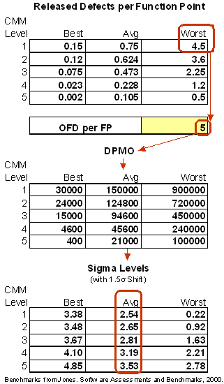
So, what is an “opportunity” in a software environment? Let’s look again at the released defect benchmarking data previously quoted from the work of Capers Jones (Figure 2). The upper table shows released defects per delivered function point for a sample of project teams at CMM levels 1-5. The upper right corner of that table summarizes a worst-case scenario for a software process, where teams in that group inserted and released about as many defects per function point as are possible. It follows that each function point must contain at least 4.5 opportunities to count defects. For simplicity, the round number of 5 OFD per function point is used going forward for discussion purposes.

The center table in Figure 2 uses the hypothetical 5 OFD per function point to convert the released defect values to DPMOs.

To understand the bottom half of Figure 2, an overview of the steps used to convert DPMO rates to Sigma levels is necessary.

Converting DPMO Rates to Sigma Levels

Sigma level definitions are framed within the presumption of a normal- or bell-shaped distribution. For situations where the defect data does not display a normally distributed curve, Sigma levels are still applicable as the conversion is based on a mathematical analogy.

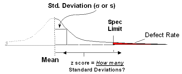
DPMO represents a defect rate and is illustrated by a specific area under the tail of the Normal curve (Figure 3). In Figure 3, the specification limit, which is set by the client, helps identify the defect area. A Sigma table (also called a Z table) is used to determine the number of standard deviations from the mean necessary to equal the DPMO defect rate. The smaller the defect rate, the larger the Sigma value or Z score.

1.5 Sigma Shift

When monitoring and controlling a process there is almost never the ability to capture and measure all output data. Instead, sampling and some form of statistical process control (SPC) are used to represent the total population. The concept of a 1.5 sigma shift was created by the founders of the Six Sigma methodology and is built on the mathematical calculations associated with SPC.

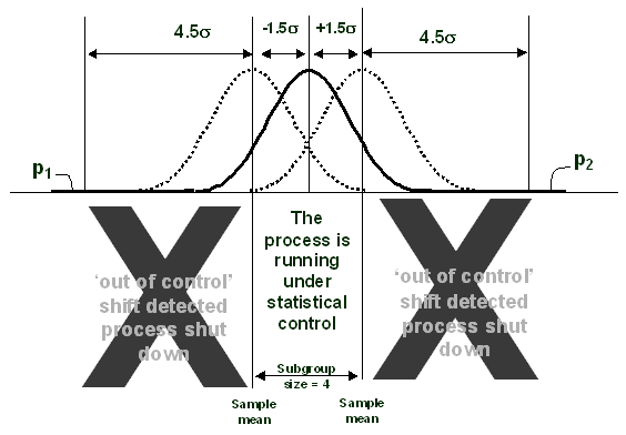
The object of the shift is to standardize a common SPC scenario where sample averages from subgroups of size 4 are periodically drawn and plotted from a stream of process data. SPC control limits, typically set at +/- 3 standard deviations, are one trigger used to decide whether or not the process is allowed to keep running. When the subgroup size equals 4, these control limits represent +/- 1.5 standard deviations of the individual process data points. Figure 4 illustrates that case.

Analyzing a process at any given time presents one of the following:

1. A best-case where the process mean is on center
2. A worst-case where the process mean has shifted 1.5 Sigma

Typically, defect data collection presumes worst-case conditions (a shifted process) requiring an addition of 1.5 to the Sigma level. When translating a Sigma level to a defect rate, assume a worst-case condition and subtract 1.5 to estimate the defect rate for the shifted case.

Checking Sigma Levels for Software Benchmark Data

The lower part of Figure 2 provides calculations of Sigma levels using the DPMO analogy and 1.5 Sigma shift. Under the calibrating assumption of 5 OFDs per function point, the average Sigma level benchmarks in the lower table run from about 2.5 to 3.5, a reasonable range.

Table 1 illustrates how the goals of this series “start simple” with the fundamental need to reduce released defects, progressing to more sophisticated goals found in this final article of the series. Each goal builds on prior work and understanding.

Invitation to Dialogue

The hope is that this discussion was instructive about Six Sigma concepts and the considerations involved in opportunity counting and Sigma levels. While our limited benchmark sample can’t argue for the broad applicability of the OFD calibration it should provide a starting point for further discussion. The author, and iSixSigma invite dialogue and other benchmark checks on the reference points presented here.