Part 1: Bottom-up Project Duration and Variation Prediction.

A number of recent posts in the iSixSigma Software Forum have inquired about the application of Six Sigma methods to Software Project Management. In particular, how might we look at software project duration as a key project-planning and execution output (a “Y” in common Six Sigma terms), to better understand the contributing factors (the “X’s”) that drive it? Learning to reduce project duration could be one goal (“reducing the mean”), but it could be more important to reduce the predicted-to-actual project duration gap (“reducing the variation”). That gap is a particularly familiar enemy in the software world, causing problems with project cost, disappointed customers, conflicts with management, development team morale, and more.

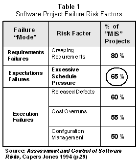Industry data from sources like Capers Jones (Table 1) show this to be an important topic, indicating that what we might call “Expectations Failures” are high on the list of contributors to software project failure. Problems related to mismatched expectations between a development team, its management, and internal or external customers show up here just under ‘Requirements Failures” (the proper subject for a number of other articles).

With the goal of reducing the gap between predicted and actual project completion times, we will begin by focusing on the process that delivers a project completion time estimate. Inaccuracies in that estimating process could, of course, contribute significantly to our completion time gap before work on the project has even started. Later, to find other “X’s” that could strongly influence the size of the “Expectation gap”, we will look for factors in play during project execution: some under the control of the project leader and team; some controlled by management; and some “uncontrolled” variables in the project environment.

We will approach this broad topic in two parts. This part will concentrate on “bottom-up” estimating methods, which will establish a good foundation for the task-level view and the methods that use it to produce forecasts. In Part 2, we will explore “top-down” estimating methods that develop predictions based on properties of the work-product, the project team, and the project environment. Throughout we will use data from several working case studies, taken from real projects and representative of what you might expect to see in actual practice.

Project Duration Estimating Process (Bottom-Up)

For best practices in project planning and management, Six Sigma practitioners are wise to leverage the toolkit and experience base that has been developed by the Project Management Institute and its “Project Management Body of Knowledge” (PMBoK). Leaving the details at the other end of those links, we will briefly outline what is involved in getting a meaningful estimate of project duration.

1. Developing the Work Breakdown Structure and Task-Level Estimates

The first step involves breaking the total project into a set of tasks, each small enough that one can answer these questions:

• What’s involved in getting started?
• How will personnel and resources be allocated, and
• What, exactly, are the conditions to be met in order to be “done”?

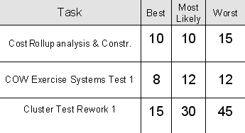
While it may be tempting to fix a “point estimate” on the duration of any task, a windowed estimate is more realistic:

2. Identifying Predecessor-Successor Relationships and the Critical Path

As tasks are evaluated for their levels of dependency on other tasks, they can be organized into a chain or network that illustrates one or more feasible plans for progressing through the whole set of tasks. Gantt Charts and Critical Path Diagrams illustrate these kinds of progressive task layouts. Figure 2 shows a simple case with seven tasks (A through F), each with a “Most Likely” duration shown in the task box.

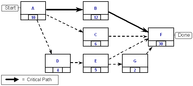
From the point of view of duration estimation, the question is, of course, “How long will it take to get everything done?” The ‘”Critical Path,” highlighted in Figure 2 is, in simple terms, the longest of all potential routes through the task network. Stated differently, the “Critical Path” is long enough to ensure that all other project tasks could be completed in parallel (assuming that required resources are available). For that reason, the critical path tasks represent a good sample for completion time estimation. Changes in the durations of critical path tasks are directly reflected in the overall project completion time. The dynamics connected with the critical path should track pretty well with the top-level dynamics of the overall project.

3. Forecasting Completion Time

With the critical path identifying the subset of all tasks to consider, practitioners typically select one of three approaches to build the completion time forecast:

• Simple ApproachAdd up the “Most-Likely” estimates for each task. While it may seem obvious that this approach fails to account for the Best and Worst estimates for each task, some software and some users still use it. The “Most Likely” estimates for the 49 tasks in our working case total 268 days. We’ll contrast that result with the others as we work them through.
• Rolling Up Task Expectation Values and VariancesThis method attempts to account for the influence of all the values in each task estimate window while assessing the variation ‘stackup’ that accumulates over the entire set of tasks. The calculations at the task level are typically done as follows:In Equation 1 (sometimes called the “PERT equation” since it may be used in PERT Charts), the expectation weights the “Most Likely” estimate by a factor of 4, while factoring in the “Best” and “Worst” estimates at face value. This skews the expectation in a way that responds to some degree to the shape of the estimation window.The variance estimate (Equation 2) assumes that the range of the task estimate window represents approximately 99% of the cases, or +/- 3 standard deviations. One sixth of that span can be used to approximate the standard deviation. Squaring that value gives an estimated variance.Table 2 illustrates these computations for several of the 49 tasks in our working case.

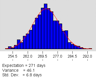
Summing the Expected Values for each task gives an expected overall project completion time. In this case, the sum for the 49 tasks on the critical path is 271 days. Using the knowledge that the variances for a series of independent events are additive, the overall completion time variance is simply the sum of the individual task variances (about 46 in this case). Figure 3 illustrates the completion time estimate as a distribution with a spread that spans from about 254 days to about 290 days.

• Monte Carlo Monte Carlo refers to an approach that uses the distribution of each “input variable” (in this case, each task-level estimate) as the basis for a simulation and draws a series of random samples from those distributions to build a set of hypothetical result values. Without any other underlying math, the simple process of input variable sampling produces a distribution of output variables that can be used as an indicator of what one might expect to see.

Setting “Assumption” Variables

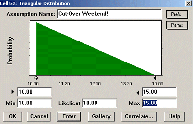
Tools like the commercial software package Crystal Ball from Decisioneering make it easy to set up and assess Monte Carlo simulations. A few examples from the case study will illustrate. First, the distribution of each input (called “Assumption”) variable is defined, using a representative distribution and appropriate parameters. Figures 4 and 5 show the way that setup is accomplished using Crystal Ball.

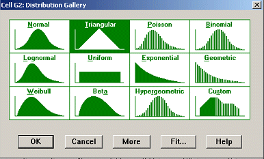
For the type of variation we expect to see in these task estimate windows, the most typical distribution choices are “Triangular” and “Beta.” We’ll use Triangular as the best simple illustration.

Figure 5 shows the triangular distribution for the first task in our case: Best and Most Likely = 10 days, Worst = 15 days. (Note that these are defined as “Min”, “Likeliest” and “Max” in Figure 5)

In a Monte Carlo setup, all other estimates are defined with the corresponding shape that the window values dictate.

Setting Forecast Variables

Another step in the setup is to define one or more forecast variables, which describe the way the predefined input variables will generate the forecast. In this case, the forecast is simply the sum of the 49 (Triangular-distributed) critical path task-level “Most Likely” values.

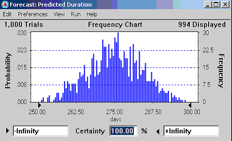
Running the simulation generates a number of graphs and statistical reports. Figure 6 shows the basic frequency chart for predicted duration.

Assessing the Probabilities Associated with Particular Completion Times

Both the Expectation Values and Monte Carlo methods allow us to calculate the likelihood that the project will be completed before or after some time point or range. With Crystal Ball, that is accomplished by moving sliders within the frequency distribution window, as illustrated in Figure 7.

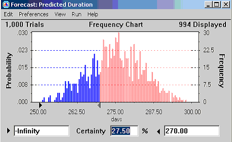
Compare the Monte Carlo appraisal with the “Simple” method in regards to the chances of meeting a 270 day deadline. The simple approach added “Most Likely” estimates to yield a project completion forecast of 268 days – suggesting we could make the 270 day deadline. Monte Carlo delivers the more sobering message that our chances may be slim indeed – less than 30%.

The Expectation and Variance method can be used to make similar predictions. With this method, an approximation to a Normal distribution is often assumed, allowing the use of Z tables to calculate probabilities.

Comparing the Three Bottom-Up Estimation Methods

We see that the simple “add-em-up” method was most optimistic (268 days) but had no defined frequency distribution connected with the forecast. The Expectation and Variance approach was more conservative (271 days) and supplied an estimate of variation (Std. Deviation = 6.8 days) as well as a target value for project completion. The Monte Carlo method was most conservative, with a project duration estimate of about 275 days and an estimated standard deviation of about 8.9 days.

These differences are not surprising, since there are quite a number of tasks with skewed estimation windows; i.e., the “Most Likely” estimate is the same as either the Best or Worst. (In our study, more of the tasks favored the “Worst” estimate.) The computation used to build the Expectation for each task weights the extreme values only by a factor of 1 (Equation 1), thereby limiting their influence on the outcome. During Monte Carlo simulation, enough events representing task times near the edges of those estimate windows showed up in the mix to pull the forecast distribution a little further in the “Worst” direction.

In practice, if most tasks are balanced (e.g., isosceles triangles), the Expectation and Variance and the Monte Carlo approaches will tend to agree. As more task estimates become increasingly skewed (e.g., right triangles), the two methods will diverge; the Monte Carlo method will pay more attention to the extremes. Bear this in mind as you explore the use of these tools. Of course, it is often possible, and advisable, to run two or more of these approaches, comparing results and interpreting the estimates on their merits for the specific case at hand. As we will show in Part 2 of this article, no one estimate can be meaningful enough to trust in isolation. A group of estimates from different perspectives can, however, advise and inform us against the backdrop of all our other experience. Together they help illuminate blind spots and steer us clear of some of the common traps.

Looking Ahead to Part 2

We will explore top-down project estimation, looking at the way commercial or custom software estimating models work and considering how such models can be calibrated and tailored for specific development environments. This discussion will bring into play some of those “other X’s” connected with the project team and the management environment as they may influence the size and nature of our decided enemy in this article set – the software project delivery “Expectations Gap.”

Part 2 > Top Down Project Effort, Duration, and Defect Prediction