Key Points
- Mood’s Median Test is a non-parametric test for testing medians between multiple samples.
- It is an alternative to other 1-way ANOVA tests.
- It isn’t the most robust test for testing, but serves a purpose due to its quick calculations.
When comparing the average of two or more groups with the help of hypothesis tests, the assumption is that the data is a sample from a normally distributed population. That is why hypothesis tests such as the t-test, paired t-test, and analysis of variance (ANOVA) are also called parametric tests.
Nonparametric tests do not make assumptions about a specific distribution. If assumptions do not hold, nonparametric tests are a better safeguard against drawing wrong conclusions.
The Mood’s median test is a nonparametric test that is used to test the equality of medians from two or more populations. Therefore, it provides a nonparametric alternative to the one-way ANOVA. The Mood’s median test works when the Y variable is continuous, discrete-ordinal, or discrete-count, and the X variable is discrete with two or more attributes.
When to Use Mood’s Median Test
Examples for the usage of the Mood’s median test include:
- Comparing the medians of manufacturing cycle time (Y) of three different production lines (X = Lines A, B, and C)
- Comparing the medians of the monthly satisfaction ratings (Y) of six customers (X) over the last two years
- Comparing the medians of the number of calls per week (Y) at a service hotline separated by four different call types (X = complaint, technical question, positive feedback, or product info) over the last six months
A Project Example
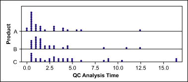
A project team wants to determine what drives the lead times of quality control (QC) analyses. One potential X they analyze is the products (A, B, C). Thus, they collect the data of all analysis times over the last three months. A dot plot (Figure 1) of the data shows a lot of overlap between the lead times of the three product groups, but it is hard to tell whether there are significant differences.

The team decided to use a hypothesis test to determine if there are “true differences” between the three product types or simply random differences due to the samples taken.

The team now has the choice between the nonparametric Kruskal-Wallis and the Mood’s median test. Because the latter is more robust against outliers and some extreme values are observed in the QC data, the team decided to use Mood’s median test.
The null hypothesis, H0, is: The samples come from the same distribution, or there is no difference between the medians of the three products’ analysis times.
The alternative hypothesis, Ha, states: The samples come from different distributions (i.e., at least one median is different).
Although the Mood’s median test does not require normally distributed data, that does not mean that it is assumption-free. Mood’s median test assumes that the data from each population is an independent random sample and that the population distributions have the same shape.
Putting It In Use
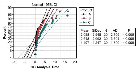
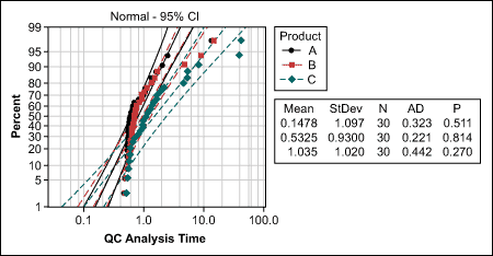
Testing for the same shape can ideally be done with the probability plot. A practitioner would now look for a distribution that is the same for all three product groups.
In this case, the probability plot (Figure 3) shows that all data follows a lognormal distribution (p>0.05), which is also typical for cycle time data. If the probability plot does not provide a distribution that matches all groups under comparison, a visual check of the data may help. Do the distributions look similar (e.g., are they all left- or right-skewed, with only some extreme values)?

If the assumptions are met, the Mood’s median test can be conducted. If the p-value is less than the agreed Alpha risk of 5 percent (0.05), the null hypothesis is rejected and at least one significant difference can be assumed. For the QC analysis time, the p-value is 0.016 – in other words, less than 0.05.
The 95 percent confidence intervals of the individual group medians now help to find where the significant difference is. The rule is: If there is no overlap between the confidence intervals, a significant difference can be assumed. In this example, at least products A and C have significantly different analysis times (Figure 4).
| |||||
Why It Matters
Mood’s Median Test isn’t perfect, but very few tools are. However, what makes this such a useful tool to consider is the speed at which you can test your null hypothesis. You need minimal data points when compared to more robust tests, which allows for fast calculations. That said, you’ll likely want to consider running a Kruskal-Wallis Test if you need more actionable data.
How the Mood’s Median Test Works
The test statistic of Mood’s median test is based on another well-known hypothesis test: the chi-square test. This test is usually used to find differences between the proportions of two or more groups. But how can it be used to compare medians?
First, practitioners should aggregate the original data into a two-way table following this procedure:
- Calculate the overall median of all the data (here: 1.66)
- Calculate the number of observations per group less than or equal to the overall median and greater than the overall median. Note that only groups containing two or more observations are included in the analysis. If there are relatively few observations greater than the median due to ties with the median, then observations equal to the median may be counted with those greater than the median.
- Display the data with a two-way contingency table (Table 1).
| Table 1: Two-way Contingency Table | |||
| Overall median = 1.66 | Product Type | ||
| Number of Observations… | A | B | C |
| Less than or equal to the overall median | 20 | 16 | 9 |
| Greater than the overall median | 10 | 14 | 21 |
The assumption (or null hypothesis) is that if there were no median difference between the groups, the percentage of values below and above the overall median should be equal for each group. The chi-square test can now be used to test this assumption. Low values of chi-square would prove this assumption true; large values would indicate that the null hypothesis is false.
In this project example, the chi-square value is 8.27. The p-value of 0.016 indicates that the probability that such a chi-square value occurs if there are no differences between the product type groups is only 1.6 percent. Therefore, the practitioners can conclude that there is at least one significant difference between the groups, with just a 1.6 percent risk of being wrong.
Other Useful Tools and Concepts
Looking for some other ways to supercharge your hypothesis testing? Learning how to make full of the two-proportions test is a great way to account for defects in your production without having to do a full 100% inspection of the entire output.
Further, learning how to make use of the Anderson-Darling Test when constructing your assumptions is a fantastic way of using data that might not fall within a normal distribution.