
Key Points
- A two-sample t-test compares significant or random differences between two samples.
- It is most useful for hypothesis testing, letting users see if an assumption is correct.
- The two-sample t-test is one of the most powerful tools you have for
The two-sample t-test is one of the most commonly used hypothesis tests in Six Sigma work. It is applied to compare the average difference between two groups. You use it to determine if the difference is significant or if it is due instead to random chance.
It helps to answer questions like whether the average success rate is higher after implementing a new sales tool than before or whether the test results of patients who received a drug are better than the test results of those who received a placebo.
An Example of the Two-Sample T-Test
Here is an example starting with the absolute basics of the two-sample t-test. The question being answered is whether there is a significant (or only random) difference in the average cycle time to deliver a pizza from Pizza Company A vs. Pizza Company B. This is the data collected from a sample of deliveries of Company A and Company B.
| Table 1: Pizza Company A Versus Pizza Company B Sample Deliveries | |
| A | B |
| 20.4 | 20.2 |
| 24.2 | 16.9 |
| 15.4 | 18.5 |
| 21.4 | 17.3 |
| 20.2 | 20.5 |
| 18.5 | |
| 21.5 | |
To perform this test, both samples must be normally distributed.
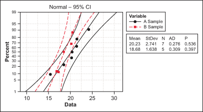
Since both samples have a p-value above 0.05 (or 5 percent) it can be concluded that both samples are normally distributed.
Testing for Normality
The test for normality is here performed via the Anderson-Darling test for which the null hypothesis is “Data are normally distributed” and the alternative hypothesis is “Data are not normally distributed.”
Using the two-sample t-test, statistics software generates the output in Table 2.
| Table 2: Two-Sample T-Test and Confidence Interval for A Sample and B Sample | ||||
| N | Mean | Standard Deviation | SE Mean | |
| A Sample | 7 | 20.23 | 2.74 | 1.0 |
| B Sample | 5 | 18.68 | 1.64 | 0.73 |
Difference = mu (A Sample) – mu (B Sample)
Estimate for difference: 1.54857
95% CI for difference: (-1.53393, 4.63107)
T-test of difference = 0 (vs not =): T-value = 1.12, P-value = 0.289, DF = 10
Both use pooled StDev = 2.3627
Since the p-value is 0.289, i.e. greater than 0.05 (or 5 percent), it can be concluded that there is no difference between the means. To say that there is a difference is taking a 28.9 percent risk of being wrong.
If the two-sample t-test is being used as a tool for practical Six Sigma use, that is enough to know. The rest of the article, however, discusses understanding the two-sample t-test, which is easy to use but not so easy to understand.
So How Does It Work?
If one subtracts the means from two samples, in most cases, there will be a difference. So the real question is not really whether the sample means are the same or different. The correct question is whether the population means are the same (i.e., are the two samples coming from the same or different populations)?
Hence, ![]() will most often be unequal to zero.
will most often be unequal to zero.
However, if the population means are the same, ![]() will equal zero. The trouble is, that only two samples exist. The question that must be answered is whether
will equal zero. The trouble is, that only two samples exist. The question that must be answered is whether ![]() is zero or not.
is zero or not.
The first step is to understand how the one-sample t-test works. Knowing this helps to answer questions like in the following example: A supplier of a part to a large organization claims that the mean weight of this part is 90 grams.
Another Example of the Two-Sample T-Test
The organization took a small sample of 20 parts and found that the mean score is 84 grams and the standard deviation is 11. Could this sample originate from a population of mean = 90 grams?

The organization wants to test this at a significance level of 0.05, i.e., it is willing to take only a 5 percent risk of being wrong when it says the sample is not from the population. Therefore:
Null Hypothesis (H0): “True Population Mean Score is 90”
Alternative Hypothesis (Ha): “True Population Mean Score is not 90”
Alpha is 0.05
Logically, the farther away the observed or measured sample mean is from the hypothesized mean, the lower the probability (i.e., the p-value) that the null hypothesis is true. However, what is far enough?
Standardizing the Sample Mean
In this example, the difference between the sample mean and the hypothesized population mean is 6. Is that difference big enough to reject H0? To answer the question, the sample mean needs to be standardized and the so-called t-statistics or t-value needs to be calculated with this formula:

In this formula, ![]() is the standard error of the mean (SE mean). Because the population standard deviation is not known, we have to estimate the SE mean. It can be estimated by the following equation:
is the standard error of the mean (SE mean). Because the population standard deviation is not known, we have to estimate the SE mean. It can be estimated by the following equation:

where ![]() is the sample standard deviation or s.
is the sample standard deviation or s.
In our example, ![]() is:
is:

Next, we obtain the t-value for this sample mean:

Finally, this t-value must be compared with the critical value of t. The critical t-value marks the threshold that – if it is exceeded – leads to the conclusion that the difference between the observed sample mean and the hypothesized population mean is large enough to reject H0. The critical t-value equals the value whose probability of occurrence is less or equal to 5 percent. From the t-distribution tables, one can find that the critical value of t is +/- 2.093.
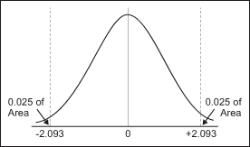
Since the retrieved t-value of -2.44 is smaller than the critical value of -2.093, the null hypothesis must be rejected (i.e., the sample mean is not from the hypothesized population) and the supplier’s claims must be questioned.
Why It Matters
When you’re doing any sort of analysis, there is a lot that goes into manipulating the data. Being able to see significant differences with a simple test is a quick way to get things done. As such, the two-sample t-test is an invaluable tool for cross-referencing samples to prove a hypothesis.
The Two-Sample T-Test Works in the Same Way
In the two-sample t-test, two sample means are compared to discover whether they come from the same population. Now, because the question is whether two populations are the same, the first step is to obtain the SE mean from the sampling distribution of the difference between the two sample means. Again, since the population standard deviations of both of the two populations are unknown, the standard error of the two sample means must be estimated.
In the one-sample t-test, the SE mean was computed as such:

Hence:

However, this is only appropriate when samples are large (both greater than 30). Where samples are smaller, use the following method:
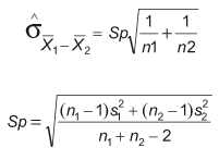
Sp is a pooled estimate of the common population standard deviation. Hence, in this method, it can be assumed that variances are equal for both populations. If it cannot be assumed, it cannot be used. (Statistical software can handle unequal variances for the two-sample t-test module, but the actual calculations are complex and beyond the scope of this article).
An In-Depth Example of the Two-Sample T-Test
The two-sample t-test is illustrated with this example:
| Table 3: Illustration of Two-Sample T-Test | |||
| N | Mean | Standard Deviation | |
| A Sample | 12 | 92 | 15 |
| B Sample | 15 | 84 | 19 |
Ho is: “The population means are the same, i.e.,![]()
Ha is: “The population means are not the same, i.e., ![]()
Alpha is to be set at 0.05.
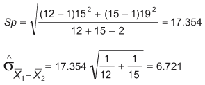
In the two-sample t-test, the t-statistics are retrieved by subtracting the difference between the two sample means from the null hypothesis, which is ![]() is zero.
is zero.
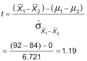
Looking up t-tables (using spreadsheet software, such as Excel’s TINV function, is easiest), one finds that the critical value of t is 2.06. Again, this means that if the standardized difference between the two sample means (and that is exactly what the t value indicates) is larger than 2.06, it can be concluded that there is a significant difference between population means.
Here, 1.19 is less than 2.06; thus, it is the null hypothesis that ![]() = 0.
= 0.
Below is the output from statistical software using the same data:
| Table 4: Two-Sample T-Test and Confidence Interval for A Sample and B Sample | ||||
| N | Mean | Standard Deviation | SE Mean | |
| 1 Sample | 12 | 92.0 | 15.0 | 4.3 |
| 2 Sample | 15 | 84.0 | 19.0 | 4.9 |
Difference = mu (1) – mu (2)
Estimate for difference: 8.00000
95% CI for difference: (-5.84249, 21.84249)
T-test of difference = 0 (vs not =): T-value = 1.19, P-value = 0.245, DF = 25
Both use pooled StDev = 17.3540
Other Useful Tools and Concepts
While we’ve discussed the two-sample t-test at length, that is only scratching the surface of tools used in hypothesis testing. First, I’d like to recommend the Anderson-Darling Test, a useful tool for assumption testing with any of your data sets.
Further, if you’re new to the world of statistical analysis, learning exactly how a normal distribution figures into your analysis is worth a read. Our comprehensive guide covers this calculation and how it applies across the board to your data.
Conclusion
The two-sample t-test is a useful means of comparing samples from two different data sets. However, it isn’t the sole tool for use when looking for variance. You’ll want to consider other tools if you’re dealing with multiple sets. However, for its intended purpose, it is a quick way of determining the mean between a pair of data sets.