Let’s face it – without meaningful data there cannot be meaningful data analysis. Data is typically collected as a basis for measuring success and, ultimately, taking action. However, unless data is viewed realistically – separating opportune signals from probable noise – the actions taken may be inconsistent with the data collected in the first place.
The context of data is the basis for the interpretation of any data set. Data can be manipulated in many ways to produce outcomes that support or oppose the subject on the table. Many times, data reported to executives is aggregated and summed over so many different processes and individual operating units that it cannot be said to have any context except a historical one – “historical” referring to the fact that the data was all collected during the same time period. With monetary figures, these aggregations may be considered rational. However, they can be extremely devastating to other types of financial data.
Before practitioners can make meaningful improvements in their financial data, they must first ensure that they are dealing with the “right” data and that they are setting goals that are within reach.
An Accounting Example
Beebe Inc., a fictitious company, has an accounting department that reconciles and closes the books for each of the operating departments within the company. Logs are kept to report on the number of hours required for each of its departments to close its books. The company’s current key performance indicators state that “on-time” closing requires fewer than 65 hours to complete. Beebe Inc.’s accounting manager, Mrs. T, has put forth a goal that 95 percent of its closings must be on time. This percentage of on-time closings is included in their monthly reports, as seen in Figure 1.

The monthly report, however, does not provide adequate context for anyone to fully comprehend or interpret the data presented. What are the trends? Are there any trends? This report does not contain enough information to determine what actions, if any, need to be taken. Once again, for example purposes, assume that Beebe Inc. has a total of 35 departments. Mrs. T captured and summarized the last 31 months of the departments’ closing activities in Figure 2.

If 35 is the maximum number of departments, then 35 would be the highest number of on-time closings that are possible. Looking at Figure 2, all departments have an opportunity for improvement, as there has not been a month wherein all 35 departments met their goal of 95 percent on-time closings.
When you look closely at Mrs. T’s direction that 95 percent of the closings should be on-time, you can see that this is actually a goal about meeting another goal, given that the true goal is to close on-time. Perhaps the manager needs to clarify more? Ninety-five percent of all departments would be 33.25 departments out of 35. If we were to ignore the 0.25 percent, then the company only met their goal for nine months out of the previous 31 months. If the manager really meant 95 percent of all closings, then we would need to look at each closing that took 65 or fewer hours to complete.
Other questions to ask: How many closings took place within each department? What if Department 2 had only two closings, of which only one closed on time? They would report only 50 percent on-time closing vs. the goal of 95 percent. In other words, the report represented in Figure 2 shows only the departments that met or exceeded 95 percent of the manager’s goal. Although this distinction may seem like hair-splitting, this data needs to be defined clearly. For this example, it should be stated that Figure 2 represents the number of departments, out of 35, that met the on-time closing goal 95 percent of the time.
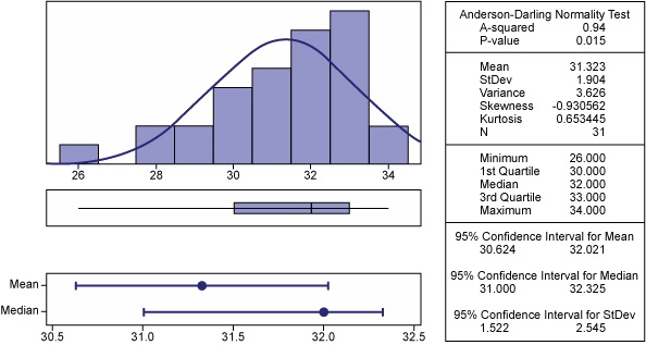
Every count has an area of opportunity. Here, the area of opportunity is the number of closings each month. If the area of opportunity remains constant over time, then you may compare the counts directly. If the area of opportunity changes from month to month, then you will have to convert the counts into rates before comparing the month-to-month values. In this example, the on-time closings data and the area of opportunity remain constant, so it is possible to work with the counts or with the percentages; the charts will tell the same story either way. A few basic statistics about Beebe’s closings are displayed in Figure 3.

The average number of on-time closings is 31.32, with a standard deviation of 1.904. The current value of 26 (shown as 74.3 percent in Figure 1) is the lowest on record. Is it a signal that something has changed, or is it simply a low value, which is part of routine variation? While displaying basic statistics is a good way to sum up the data, the simplest way to answer this question is to use a process behavior chart.
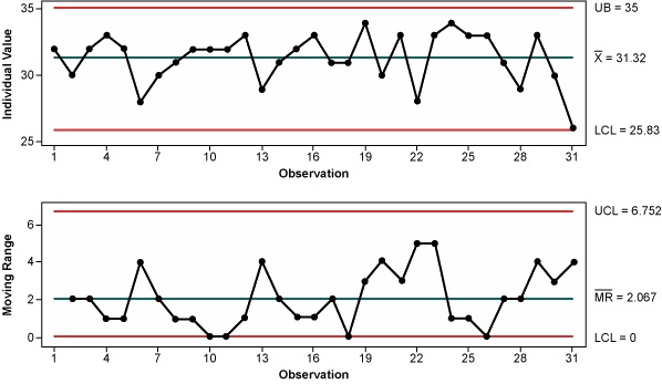
The individual moving-range (I-MR) chart for the number of on-time closings is shown in Figure 4. The limits of this chart can be based on either the values from the first two years or simply on the three standard deviations. Once again, the average number of on-time closings is 31.32. The average moving range is 2.0. There is no meaningful upper natural process limit because the maximum count is 35. The lower natural process limit would be 26.2. This example uses the three standard deviations, which will give a lower control limit (LCL) of 25.83. The upper range limit is 6.752.

The last point on the individual chart is the current value. It does not fall below the LCL; however, it could be taken to be a signal if the process’ natural lower limit truly is 26.2. Regardless, something was different about the closings in June 2010, as detectably fewer departments had their books closed on time. The process behavior chart does not indicate what happened, but it does show that something did happen and that some questions are in order.
With the exception of the June value, the on-time closings appear to behave predictably. Up until the present, the departments have averaged 31.32 on-time closings per month (90 percent on-time). This means that while they might occasionally have a month with better than 95 percent on-time closings, they cannot average 95 percent on time. This goal is beyond the capability of the system. In order to have an average that will meet this goal, the system would need to be changed in some basic way.
Charting Goals Not the Answer
Charting the on-time percentage goal will not reveal how to change the system; neither will it highlight the problem areas. Mrs. T will not be able to bring about the desired changes by setting goals for the on-time percentage. Instead of reprimanding the employees, Mrs. T must work on improving the system.
Summary counts and percentages, such as this on-time data, will never be focused and specific; they are too highly accumulated. At best, such accumulations may serve as report cards. However, because the wrong data points may be counted, or the correct counts may be accumulated in the wrong way, some accumulated measures may not even yield useful report cards.
With the on-time closings, the key to useful data comes from the realization that the closing of the books may well involve different operations and procedures for each of the 35 departments. Therefore, some departmental books may take longer to close than others. This means that process managers will need to consider the 35 closings as 35 parallel operations, each with its own stream of data: the number of hours needed each month. These 35 data streams will need to be analyzed separately in order to discover if they behave predictably or not.
If a given departmental closing displays predictable variation, then it will do no good to set a goal on the number of hours for that closing; you will only get what the system will deliver, and setting a goal can only distort the system. If a given departmental closing does not display predictable variation, there is again no point in setting a goal; the system has no well-defined capability, so there is no way of knowing what it will produce.
Instead of setting arbitrary goals, Mrs. T needs to analyze the data for the departmental closings in order to discover problem areas and opportunities for improvement.
Much of the managerial data in use today consists of aggregated counts, such as the data presented by Mrs. T. Such data tends to be virtually useless in identifying the nature of problems because the aggregation destroys the context of the individual counts. The work of process improvement requires specific measures and contextual knowledge. These characteristics are more readily available from measures of activity than from counts of events.
Developing Stronger Measures
Measures of actual activity will generally be more useful than simple counts of how many times a goal has been met. If management is serious about improvement, they will have to take the time to develop measures that help, instead of simply counting the good days and the bad days. The teams need to look back at their process and find the variables that best represent their process. In short, good data does not occur by accident; it has to be obtained by plan.