The CLT allows you to use sample data to make inferences about your population. If you take a large enough sample and plot the means of the samples, you will form a distribution of sample means with some interesting characteristics. Let’s explore those in more detail.

Overview: What is the Central Limit Theorem (CLT)?

One of the problems of inferential statistics is that using sample statistics to make inferences about population parameters will always result in some error. Unfortunately, it is not practical to measure all items in your population of data. The question is how do you mitigate that error? The CLT is one common way. The term central limit theorem was first used in the title of a 1920 paper by George Polya. Polya claimed the theorem was central because of its importance in probability theory.

In simple terms, the CLT states that if you have a population with mean (mu) and standard deviation (sigma) and take sufficiently large random, independent samples from the population with replacement, then the distribution of the sample means will approach a normal distribution.

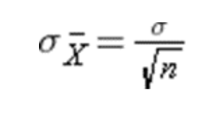
This will hold true regardless of the shape of the population distribution and the sample size is sufficiently large ( n > 30). If the underlying population is normal, then the theorem holds true for samples smaller than 30. Additionally, the mean of the sampling distribution will approach the mean of the population as sample size increases. Finally, the standard deviation of the sampling distribution will be related to the population standard deviation as follows:

3 benefits of the Central Limit Theorem

Here are a few benefits of the Central Limit Theorem

1. Allows for assumption of normality

If you select an appropriate size and number of random, independent samples, you are assured your sampling distribution will approach normality. If you need normality for a particular statistical test then you can be confident it will be valid.

2. Applicable to both continuous and discrete data

The Central Limit Theorem can be used with continuous variable data as well as binary (binomial) and discrete (Poisson) data.

3. Effective at relatively small sample sizes

The sample size for effective use of the Central Limit Theorem of around 30-50 is sufficient to achieve normality of the sampling distribution as you collect more and more data.

Why is the Central Limit Theorem important to understand?

You will want to understand the Central Limit Theorem for the following reasons:

Assumption of normality

The Central Limit Theorem is important for statistics because it allows you to safely assume that the sampling distribution of the mean will approach normality so you can take advantage of statistical techniques that assume a normal distribution.

Flexibility of using with different distributions

Since the Central Limit Theorem can be used with both continuous and discrete data, there is flexibility as to its use in a variety of different applications.

Independent of the underlying distribution

The normality of the sampling distribution will occur regardless of the shape of the underlying distribution so you can safely sample from any distribution shape and be confident the sampling distribution will approximate a normal distribution.

An industry example of the Central Limit Theorem

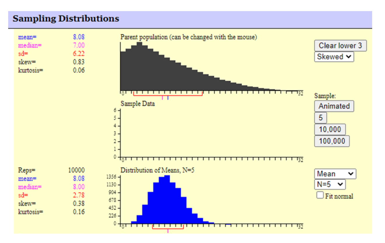
The graphic below shows the resulting sampling distribution when 10,000 samples of size 5 are drawn from a heavily skewed population distribution. Note how the mean of the sampling distribution is essentially equal to the population mean. Also, the standard deviation of the sampling distribution is equal to the population standard deviation divided by the square root of the sample size of 5 (6.22/2.236). Finally, note the shape of the sampling distribution appears to be close to normal despite the very heavily skewed population distribution where the samples were taken from.

3 best practices when thinking about the Central Limit Theorem

Here are some tips for properly applying the Central Limit Theorem.

1. Select an appropriate sample size and number of samples

Sample sizes should be around 30. The outcome of the Central Limit Theorem will improve as the number of samples you gather increases.

2. Do a Measurement System Analysis (MSA)

Since you are relying upon sample data to make your decisions, be sure you have conducted an MSA to validate your measurement system.

3. Check your normality

Since the outcome of the Central Limit Theorem is to establish a normal distribution of means, you should test whether that has occurred either with a Normal Probability Plot or a statistical method like the Anderson-Darling test.

Frequently Asked Questions (FAQ) about the Central Limit Theorem

What is an appropriate sample size for the Central Limit Theorem to work?

A sample size between 30 – 50 is sufficient for the Central Limit Theorem. A larger sample is even better but samples must be randomly selected and be independent.

Does the Central Limit Theorem work if my population is not normally distributed?

Yes, that is the underlying premise of the Central Limit. As your sample size increases, your sampling distribution will approach normal regardless of the shape of the population you are sampling from.

Will the spread or standard deviation of my sampling distribution be the same as the population?

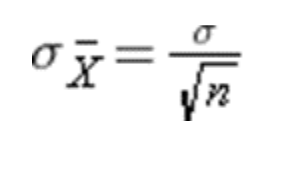
No. Since you are taking samples and plotting means of those samples, the high and low values found in your population will be dampened. Therefore, your sampling distribution will be narrower than your original population. The relationship is as follows:

Summary of the Central Limit Theorem

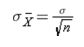
The basic assumption of the Central Limit Theorem is that if you take samples from some population and calculate the means of those samples, the distribution of those means will approach normality as the sample size and number of samples increases regardless of the shape of the population from which you sampled. Furthermore, the mean of the sampling distribution will approach the mean of the underlying population you drew the samples from. Finally, the standard deviation of the sampling distribution will be related to the population standard deviation as follows: