Even a novice on a Six Sigma project team knows each step in the basic five-step DMAIC method (Define, Measure, Analyze, Improve, Control) is essential to the success of a breakthrough project. What is not as widely recognized, however, is that each step brings a distinct set of tools to bear on the project objective. For the Analyze and Improve steps, design of experiments (DOE), combined with analysis of variance, is the Six Sigma power tool.

Design of experiments was first conceived and developed by Sir Ronald A. Fisher in the 1920s and 1930s. Fisher was a brilliant mathematician and geneticist working to improve crop yields in England. He designed and supervised field trials comparing fertilizers and seed varieties, among other things. Fisher encountered two enormous obstacles: 1) uncontrollable variation in the soil from plot to plot and 2) a limited number of plots available for any given trial. He solved these problems by the arrangement of the fertilizers or seed varieties in the field.

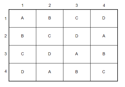
For example, to determine which of four varieties of wheat had the highest yield, Fisher would divide a rectangular test field into 16 plots. He then planted each of the four varieties in four separate plots. Each of the four varieties (A, B, C and D) was planted just once in each row and once in each column (Figure 1). This minimized the effects of soil variation in the analysis of the plot yields.

Fisher also developed the correct method for analyzing designed experiments. He called it “analysis of variance” because it breaks up the total variation in the data column into components due to different sources. Today these vector components are called “signals” and “noise.” There is a signal component for each controlled variation and a noise component representing variations not attributable to any of the controlled variations. By looking at the signal-to-noise ratio for a particular variation, the analysis of variance will provide accurate answers.

The problems Fisher encountered in conducting agricultural experiments in the 1920s exist today in virtually all Six Sigma applications. For example, industrial experimenters are confronted by significant degrees of uncontrollable variation in such areas as raw materials, human operators or environmental conditions. Such problems can be overcome by running sufficiently large experiments. Unfortunately, large experiments are often too expensive, too time consuming, or both. Fortunately, Fisher’s solutions to these problems work just as well in 21st century Six Sigma as they did in 20th century agriculture. In fact, Fisher’s methods of design and analysis have become international standards in business and applied science.

Fisher’s methods require well-structured data matrices. His analysis of variance delivers surprisingly precise results when applied to a well-structured matrix, even when the matrix is quite small.

Case Study: The Daily Grind

Don worked in the belt grinding department. Day after day, he and his co-workers removed gate stubs from metal castings to prepare them for final processing and shipping. The grinders were paid a handsome hourly rate. The other major expense was the cost of the belts. The department went through a lot of belts on a typical shift.

Define: If a belt is used beyond a certain point, the efficiency in removing metal goes way down. The supplier representative had given the area manager a rule for when the grinders should replace a worn belt. The rule was called “50 percent used up.” Examples of belts that had been 50 percent used up were hanging on the walls in the grinding department. The purpose of the rule was to minimize the total expense of the operation. Don thought the rule was wrong. He thought the rule caused them to discard the belts too soon. He had a hypothesis that using the belts a little longer would reduce the belt expense with no loss of grinding efficiency. He also suspected that the supplier just wanted to sell more belts.

Don had come up with a new rule called 75 percent used up. He proposed doing a designed experiment to determine whether or not the new rule was more cost effective than the old rule. Don, the area manager and the supplier representative discussed the project. The supplier representative was vehemently opposed to the project. He said the 50 percent rule was based on extensive experimentation and testing at his company. He said the grinding department was wasting time trying to reinvent the wheel.

Don argued that laboratory tests may not be good predictors of shop-floor performance. The area manager thought Don had a good point. He gave the go-ahead for the project. He allowed Don one full day to complete the experiment.

Measure: When the other grinders heard about the experiment, they suggested other things that could be tested in addition to the 50-versus-75-percent usage. The contact wheels currently used on the grinding tools had a low land-to-groove ratio (LGR). One of the grinders wanted to try a wheel with a higher LGR. Another wanted to try a contact wheel made out of hard rubber instead of metal (Material). A third reminded Don that belts of at least two different grit sizes were routinely used. He felt that both grits should be represented in the experiment to get realistic results (Grit).

Don figured he could get 16 castings done in one day. But he also felt that he was usually more efficient mornings than afternoons. The experiment was controlled for this by including a morning/afternoon factor in the matrix (Session). Above is the data matrix for the experiment which tested all five factors. The response variable was the total cost for each casting divided by the amount of metal removed. The total cost was calculated as labor cost plus belt cost.

Analyze: A well-designed experiment is usually easy to analyze. The data matrix suggested the following:

1. Don was on to something with his 75 percent used up
2. High LGR is better than low
3. Rubber wheels are worse than metal ones

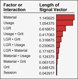
Figure 2 shows the Pareto plot ranking the factors and their interactions in the belt grinding experiment by the strength (length) of their profit signals.

The strongest signal was the comparison of steel to rubber contact wheels (Material). This signal indicated that rubber was not a good idea. The next-largest signal was the comparison of the 50 percent rule to the 75 percent rule (Usage). It predicted significant savings with Don’s idea. The third-largest signal was the comparison of low to high land-to-groove ratio (LGR) for the contact wheel.

The next two signals involved interactive effects. The message here was that the actual cost reductions from implementing the Usage and LGR results would be different for the two grit sizes.

Improve: Don’s experiment produced two recommendations: 1) use his 75 percent rule instead of the supplier’s 50 percent rule and 2) use contact wheels with the higher land-to-groove ratio. The combined impact of these two changes was a predicted cost reduction of $2.75 per unit of metal removed. This amounted to about $900,000 in annual savings.

Don’s recommendations were quickly implemented throughout the grinding department. The actual savings came in a little under the prediction, but everyone was happy. Not bad for a one-day project.

Control: Some degree of cost reduction was achieved by all the grinders, but it did not apply uniformly. There was still a lot of variability in grinder performance. Attacking this variation obviously was the next step.

Conclusion

Design of experiments and analysis of variance are hardly new, but they remain vital ingredients in virtually all applications of the Six Sigma DMAIC cycle. Good experiments require well-structured data matrices. Modern statistical software packages will generate such matrices automatically for any experiment specified. The same programs perform the appropriate analysis of variance at the click of a mouse. Thus, statistically valid comparisons and accurate predictions are now available to all, even when small experiments are demanded.

There are, of course, key disciplines in design of experiments that depend on the experimenters and not the software. These include choosing appropriate responses (output variables) and factors (input variables), setting appropriate factor ranges or levels, creating documentation for everyone involved in the experiment, managing the experiment as it takes place, reporting and presenting results, deciding whether to further optimize the process or just run a confirmation experiment. In other words, a designed experiment is a DMAIC cycle-within-a-cycle.