Six Sigma projects in various industries often deal with experiments whose outcomes are not continuous variable data, but ordered categorical data. Analysis of variables (ANOVA) is a technique used to analyze continuous experimental data, but is not adequate for analyzing categorical experimental outcomes. Fortunately, many other methods have been developed to deal with categorical experiments, such as Jeng and Guo’s weighted probability-scoring scheme (WPSS).
The WPSS technique is interpretable and easy to implement in a spreadsheet software program. The following case study, which involves medical devices, serves as an example of how a modified WPSS technique can be used to analyze experiments with ordered categorical data.
Determining the Best Factors
This study explores the influence of contact lens design factors on outcomes related to ease of lens insertion, meaning how easy it is to put patients’ contact lenses in their eyes. Soft contact lenses are thin pieces of plastic or glass that float on the tear film on the surface of the cornea. They are shaped to fit the user’s eye and are used to correct refractive errors such as nearsightedness, farsightedness and unequal curvature of the cornea (astigmatism). For this example, only three lens design factors of a certain lens type with fixed material properties are considered: lens thickness profile (3 levels), base curve dimension (3 levels) and base curve profile (2 levels). Determining the ease of insertion is a five-step process.
Step 1: Design an Experiment
Because this is an exploratory experiment, an L9 orthogonal matrix is used. The design matrix with the three lens design factors is shown in Table 1.
| Table 1: L9 Orthogonal Matrix of Three Lens Design Factors | |||
|
Design Factors |
|||
| Experiment Number | Thickness profile | Base curve dimension | Base curve profile |
| 1 | 1 | 1 | 1 |
| 2 | 1 | 2 | 2 |
| 3 | 1 | 3 | 1 |
| 4 | 2 | 1 | 2 |
| 5 | 2 | 2 | 1 |
| 6 | 2 | 3 | 1 |
| 7 | 3 | 1 | 1 |
| 8 | 3 | 2 | 1 |
| 9 | 3 | 3 | 2 |
Step 2: Plan Number of Samples and Data Categorization
In small clinical trials, nine trained contact lens wearers are asked to try each of the nine lens designs from the L9 matrix and give their opinion on the ease of insertion. Each time a patient inserts a lens in their eye, they are asked to rate how easy it was to do. Their responses are integer numbers from 1 to 10, with the worst condition rated 1 (the patient cannot insert the lens) to the best condition rated 10 (the patient needs only one trial and the lens immediately sits on the right location of the eye). The ratings are grouped into four categories of ease of insertion:
- Category I (very easy to insert): Ratings 9 – 10
- Category II (easy to insert): Ratings 7 – 8
- Category III (moderate to insert): Ratings 5 – 6
- Category IV (difficult to insert): Ratings 1- 4
The design matrix with the outcomes for each run is shown in Table 2.
| Table 2: Insertion Ratings Grouped By Category | ||||||||
|
Design Factors |
Number of Observation By Category | |||||||
| Experiment Number | Thickness profile | Base curve dimension | Base curve profile | I | II | III | IV | Total |
| 1 | 1 | 1 | 1 | 1 | 2 | 5 | 1 | 9 |
| 2 | 1 | 2 | 2 | 3 | 3 | 3 | 0 | 9 |
| 3 | 1 | 3 | 1 | 4 | 2 | 2 | 1 | 9 |
| 4 | 2 | 1 | 2 | 2 | 2 | 3 | 2 | 9 |
| 5 | 2 | 2 | 1 | 4 | 4 | 1 | 0 | 9 |
| 6 | 2 | 3 | 1 | 1 | 3 | 1 | 4 | 9 |
| 7 | 3 | 1 | 1 | 5 | 3 | 1 | 0 | 9 |
| 8 | 3 | 2 | 1 | 2 | 5 | 1 | 1 | 9 |
| 9 | 3 | 3 | 2 | 4 | 1 | 4 | 0 | 9 |
Step 3: Calculate Probability of the Outcomes Per Category and Run
In order to estimate the location and dispersion effects of each run, the scores of each category of each run must be transformed into probability values. Let i be an experiment run, for i = 1, 2,…I (in this example, I = 9) and j be a category of experimental outcomes, for j = I, II,…J (in this example J = IV). Then it is possible to calculate the probability (proportion) that an outcome is placed in j-th category of i-th run, i.e. pij, as the following:
pij = nij/si
where nij is the number of outcomes in j-th category of i-th run and si is the total outcomes of all categories in the i-th run.
For example, the probability of an outcome being placed in the III-th category of the 1st run is p1III = n1III/s1 = 5/9 = 0.56. The probability of the outcome in each category of each run is shown in Table 3.
| Table 3: Probability of Outcomes | |||||||||
|
Number of Observation |
Probabilities for Each Category |
||||||||
| Experiment Number | I | II | III | IV | Total | (I) | (II) | (III) | (IV) |
| 1 | 1 | 2 | 5 | 1 | 9 | 0.11 | 0.22 | 0.56 | 0.11 |
| 2 | 3 | 3 | 3 | 0 | 9 | 0.33 | 0.33 | 0.33 | 0.00 |
| 3 | 4 | 2 | 2 | 1 | 9 | 0.44 | 0.22 | 0.22 | 0.11 |
| 4 | 2 | 2 | 3 | 2 | 9 | 0.22 | 0.22 | 0.33 | 0.22 |
| 5 | 4 | 4 | 1 | 0 | 9 | 0.44 | 0.44 | 0.11 | 0.00 |
| 6 | 1 | 3 | 1 | 4 | 9 | 0.11 | 0.33 | 0.11 | 0.44 |
| 7 | 5 | 3 | 1 | 0 | 9 | 0.56 | 0.33 | 0.11 | 0.00 |
| 8 | 2 | 5 | 1 | 1 | 9 | 0.22 | 0.56 | 0.11 | 0.11 |
| 9 | 4 | 1 | 4 | 0 | 9 | 0.44 | 0.11 | 0.44 | 0.00 |
Step 4: Estimate Location and Dispersion Effects of Each Run
Given each category j has a weight wj, which is the upper limit of the j-th category rate, the location scores Wi for the i-th run is defined by:
![]()
The rationale for using the upper limit of the category rate is that the weight should reflect the rating values. The dispersion score di2 is defined by:
![]()
where the target values are defined as {The upper limit of the I-st category rate, 0, 0, …, 0} for categories {I, II, III, … ,J}, respectively.
The rationale of setting the target values is that only outcomes that fall in the best category are rewarded. For example, the location and dispersion scores for the 1st run are W1 = 10*0.11 + 8*0.22 + 6*0.56 + 4*0.11 = 6.7 and d12 = [10*0.11 – 10]2 + [8*0.22 – 0]2 + [6*0.56 – 0]2+ [4*0.11 – 0]2 = 93.48. The location and dispersion scores of the outcomes of each run are shown in Table 4.
| Table 4: Location, Dispersion and Mean Square Deviation Scores | ||||||
| Experiment Number | Design Factor – Thickness Profile | Design Factor – Base Curve Dimension | Design Factor – Base Curve Profile | Location Scores (Wi) | Dispersion Scores (di2) | MSD |
| 1 | 1 | 1 | 1 | 6.7 | 93.5 | 0.16 |
| 2 | 1 | 2 | 2 | 8.0 | 55.6 | 0.06 |
| 3 | 1 | 3 | 1 | 8.0 | 36.0 | 0.04 |
| 4 | 2 | 1 | 2 | 6.9 | 68.4 | 0.11 |
| 5 | 2 | 2 | 1 | 8.7 | 44.0 | 0.04 |
| 6 | 2 | 3 | 1 | 6.2 | 89.7 | 0.21 |
| 7 | 3 | 1 | 1 | 8.9 | 27.3 | 0.03 |
| 8 | 3 | 2 | 1 | 7.8 | 80.9 | 0.08 |
| 9 | 3 | 3 | 2 | 8.0 | 38.8 | 0.04 |
One performance measure to combine location and dispersion effects is mean square deviation (MSD), which allows practitioners to make judgments in one step. If any outcome is the larger-the-better characteristic, then its expected MSD can be approximately expressed in terms of location and dispersion effects as follows:

For example, the expected MSD for 1st run is E[MSD]1 = 1/(6.67)^2 (1+ (3*93.5)/(6.67)^2) = 0.16. The MSD scores for all runs are given in Table 4.
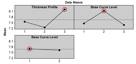
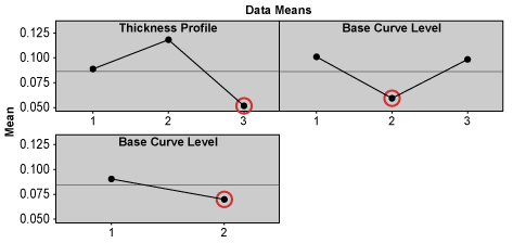
The location, dispersion and expected MSD effects for each design factors are shown as Tmax-Tmin (Figures 1, 2, 3). Higher Tmax-Tmin values or steeper main effects curves indicate a stronger influence of that design factor on the outcomes.

|
|||||||||||||||||||||||||||||||||

|
|||||||||||||||||||||||||||||||||

|
|||||||||||||||||||||||||||||||||
Step 5: Determine Optimal Solutions
The level of a particular design factor with the highest location value, the lowest dispersion value or the lowest expected MSD value is the optimal solution for each of those factors, respectively. The optimal solution based on the expected MSD criteria is the optimal trade-off between maximal location and minimal dispersion scores.
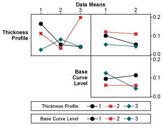
The predicted optimal solution based on the expected MSD criteria is thickness profile at level 3, base curve dimension at level 2 and base curve profile at level 2. But if practitioners know there are interaction effects among design factors, they cannot depend solely on the main effect values or plots to choose the settings of design factors. The interaction plot for the expected MSD effects shows that thickness profile heavily interacts with base curve level/dimension (Figure 4). A small interaction also exists between base curve dimension and base curve profile. After taking interaction effects into consideration, practitioners need to examine whether the chosen optimal design factor levels still give optimal effects to the experiment outcomes.

In this case, thickness profile at level 3 gives almost consistently the lowest MSD scores for different levels of base curve dimension and also consistently gives the lowest MSD scores for different levels of base curve profile. Thus, it gives the optimal effect to the experiment outcomes. Base curve dimension at level 2 almost consistently gives the lowest MSD scores for different levels of thickness profile and also consistently gives the lowest MSD score for different levels of base curve profile. Thus, it too gives the optimal effect to the experiment outcomes. The Tmax-Tminvalue of the base curve profile is the lowest and its curve is flat. Thus, base curve profile has insignificant influence on the outcomes, and can be set at either level 1 or 2. Therefore, the expected MSD predicts that lens design with thickness profile at level 3, base curve dimension at level 2 and base curve profile at either level 1 or 2 would give the optimal ease of insertion.
Easy to Implement Optimization Method
A modified WPSS is a simple and straightforward method for dealing with ordered categorical data. This case study shows that a single performance measure MSD derived from WPSS can provide insight to a system through experiments and can direct practitioners to the optimal solution.