Well-focused improvements done in the right place can lead to significant system-wide results for an organization. In simple terms, it is a matter of choosing the right Six Sigma projects. But the problem is that it is not always easy to know which projects will produce the highest system-level leverage.

Often Green Belts and Black Belts are left to their own devices to find projects. Because the locus of high-leverage changes is normally not located in close proximity, either in time or space, to the symptoms of the problem, it is often not obvious to participants in the system. The result is the “right” projects may not be selected.

Pursuing projects that do not have high leverage may result in local optimization but have little or no effect in the global system. Unfortunately, the current Six Sigma body of knowledge does not contain any method of thinking that teaches Belts to locate areas of high-leverage changes.

Another potential project selection problem is sub-optimization, which is the result of negative leverage projects. It occurs when a part of the system is optimized but the larger system is worse off as a result. A well-known example of this in the Lean literature is over-production. Over-production is the result of efforts by a part of the organization to optimize its processes without realizing that the larger system has no immediate use for the additional production.

Sub-optimization can be a real threat for the viability of Six Sigma programs. Organizations embarking on Six Sigma need a methodology to understand the global dynamics of the larger system to facilitate global optimization through local projects.

Example of Linear Cause-and-effect Thinking

Here is an example of what can happen with cause-and-effect thinking in a linear world. Imagine a Web-based laptop firm which has as its key value proposition the ability to offer a highly customized product to the customer’s doorstep at a competitive price. The company is able to do this largely because it only orders product parts and commences production only after it has received a paid customer order. The company has experienced phenomenal growth in the last three years. Website traffic is climbing to an all-time high and sales have doubled.

However, all is not rosy. Profitability has dropped, which the CEO thinks is largely a pricing issue. In addition, customers are starting to complain about product quality. And more customers are finding it difficult to get on the company’s technical support helpline. Calls to the helpline have increased by 300 percent in the last year and the call center is only able to handle about 50 percent of the calls.

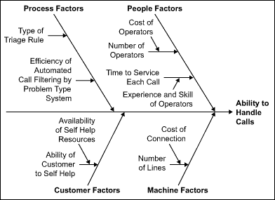
The CEO tasks a Six Sigma Black Belt to fix the call center problem, and wants 98 percent of all calls to be answered within three rings. As in any typical Six Sigma project, one of the first steps is a cause-and-effect analysis. The project team led by the Black Belt comes up with a fishbone diagram similar to the example in Figure 1. Eventually, the team finds the following: 

• The availability of operators has a significant effect on the ability to handle the call volume. Data gathered indicates that there is a pattern to the call volume. So the team redesigns the work schedule to allocate more resources for high volume hours.
• Customers typically hang up after two minutes if they do not get through to an operator. To solve this problem, after 1.5 minutes callers are given an option to leave their phone number and have operators get back to them during off-peak hours. This list of customers is monitored daily to ensure that everyone is in fact called back.
• Some operators are spending significantly more time with customers than other operators are. To solve this, the team identifies the 20 most common customer concerns and give operators scripts to follow in those situations. The extra time being spent disappears within a month of implementation. 

In addition, the team finds that 45 percent of customer problems could easily be resolved by customers themselves if they only knew how. The team recommends the creation of an online self-help system for customers. And, an improved problem classification system allows the company to transfer all low-complexity problems to an outsourced call center in the Philippines. 

With this array of solutions, the team manages to move the call answering rate to 75 percent and the project is pronounced a resounding success. But is it really a success? 

Cause-and-effect Thinking from a Systems Perspective

System dynamics or systems thinking was pioneered by Jay W. Forrester and popularized by Peter Senge in his book, The Fifth Discipline. The book title refers to the discipline of systems thinking, which Senge says is a necessary component of “learning organizations” – organizations that can “learn” in order to continually enhance their own capabilities. In a nutshell, systems thinking takes cause-and-effect thinking to a higher level and encourages the user to see not just the linear causal connections but also the web of causal interconnections that come into play in real systems. The representation of these causal interconnections is called a causal loop diagram (CLD).

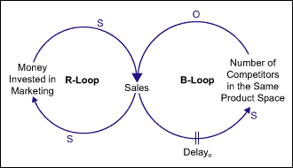
In CLDs and in real life, there are only two possible relationships between two related variables: The first relationship is “moving in the same direction.” An example is when a company invests in marketing, generally sales increase. This relationship is called “same,” or “s” for short. The second relationship is “moving in the opposite direction.” An example is when the number of competitors grows, a company’s sales normally go down. This relationship is called “opposite,” or “o.” Both examples are illustrated in Figure 2. In Six Sigma, these relationships are considered either positive correlation or negative correlation. 

Building Blocks of CLDs – Reinforcing and Balancing Loops

Causal loop diagrams attempt to move away from linear cause-and-effect thinking toward dynamic closed loop thinking. This allows a study team to see how parts of the larger system being mapped might interact to generate problems even if these variables are separated by time and space. By understanding these global dynamics, a good CLD can lead a study team closer to a higher leverage solution area compared with a team that merely relies on linear cause-and-effect mapping. 

The first type of causal loop that is often encountered in nature and in organizations is the reinforcing loop, or R-loop.

Figure 2 is an R-Loop example: When more money is invested in marketing, sales increase and when sales increase, more money gets invested in marketing and so sales increase and so on. The opposite is also true. When less money is invested in marketing, sales drop and when sales drop, less money gets invested in marketing. This is the so-called “vicious circle,” or more politely, engines of growth or collapse. In a time series plot, this type of dynamics will generate either an exponential upward or downward curve. 

The second type of causal loop is the balancing loop or B-loop. Balancing loops basically acknowledge that nothing grows or collapses forever. Balancing loops are stabilizers. They are the part of the system that causes the familiar regression-to-the-mean effect. Balancing loops resist change in one direction by producing change in the opposite direction. 

The configuration of a growth R-loop paired with a limiting B-loop is called “limits to growth” (Figure 3). It is a common phenomenon that with every growth engine, over time, a B-loop will be acting to constrain it. In the case of the laptop firm, the limit-to-growth story goes like this: Imitators see the viability of the laptop company’s business model and they develop their own internal capabilities to support such a business model and offer it to the market. For instance, Dell was the first computer manufacturer to offer build-to-specification Internet ordering in the computer business, but today all major computer manufacturers offer the same thing.

The R-loop and the B-loop are building blocks of all CLDs. By modeling the dynamics in the case study, it is possible to determine what project should have been deployed to offer the highest potential leverage.

Mapping the Case

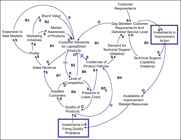
The causal loop diagram in Figure 4 clearly contains a lot more information than the fishbone analysis. It looks complicated at first, although it is built of nothing but R-loops and B-loops. The first question most people ask is how does one figure out which is an R-loop and which is a B-loop? There is both a simple way and the correct way of finding out. The simple way is to count the number of “o” links. If there are none or if there are an even number of them, it is an R-loop; otherwise it is a B-loop. The correct way is to trace the path using logic to see if the effect on the outcome variable is growth/collapse or balancing. 

What should become clear after studying the CLD is that the choice for management is to invest in either fixing quality problems or fixing the call center process. What is more interesting is the mapping that shows that improvement resources are finite and that investments in fixing the call center process draws resources away from the efforts to fix the underlying quality. 

Simplify the CLD and a system archetype called “shifting the burden” is encountered. This is a fairly common organization issue: Should a problem be addressed by applying a symptomatic solution (fix the call center) or a more fundamental longer-term solution (fix the quality problems)? What is most damaging about applying the symptomatic solution is that when resources are drawn to implementing the symptomatic solution, the symptoms go away (ability to handle customer complaints goes up) and this diverts attention away from the fundamental solution, which makes attempts to solve the real problem more difficult. 

In this case, the higher leverage intervention is to fix the quality problems because it is the source of all other problems. Fixing the quality problems will remove the need to fix the call center problem because demands for technical support will drop. A Six Sigma project team that understands the larger system dynamics through CLD mapping will have a better chance to solve high leverage problems. In this case, the Black Belt might have (if there were enough resources), launched two project clusters – one to alleviate the call center problem because of its immediacy and a large project cluster to address the quality issues. In this way, the organization could resolve both its immediate problem and the more fundamental problem and stay in business. 

Conclusion: Systems Thinking Integrates with Six Sigma

Systems thinking has the potential for some interesting applications during the Six Sigma journey: 

• A company’s leadership team can use systems thinking in order to kickoff a high-impact initiative by focusing on real root cause areas rather than the symptoms of high level problems.
• A Master Black Belt can use systems thinking to map out the system dynamics around a mission critical Big Y that he or she has been tasked to optimize, and then identify the various high-leverage daughter projects.
• A Black Belt or Green Belt can use systems thinking during the Define phase to identify the possible negative consequences of optimizing the project Y. By doing so, the project team can strategize how to avoid, eliminate or minimize these negative consequences. For instance, when trying to optimize end-to-end process flow time, one typical negative consequence is the reduction of quality.
• A Black Belt or Green Belt can use systems thinking during the Measure or Analyze phases to identify the system dynamics of the critical Xs that affect the project Y that the team has been tasked to optimize. 

Six Sigma programs can avoid irrelevance by addressing the real issues of an organization with the use of systems thinking. It would be another step in integrating successful management practices into a single management system which wisely uses resources while focusing on what is important for customers, shareholders and employees.