Six Sigma’s positive impact on manufacturing and product quality environments is well known and, without a doubt, has been proven by countless early and present practitioners. The method’s usefulness in improving transactional processes even in manufacturing businesses, however, is not always so well accepted. At Cabot Microelectronics Corporation, the business forecasting process was one that most in the company seemed to agree, could not be improved. However, applying the Six Sigma methodology and tools produced impressive results. And reaching into other toolboxes can bring additional value to process improvement activities as well.

In the Beginning and Then…

When the company initiated the use of Six Sigma, it began looking around the business at the key drivers of cost, the typical heavy hitters showed themselves early on. Poor product quality, poor raw material quality, labor inefficiencies and logistics costs were the low hanging fruit that made obvious the initial Six Sigma projects.

Once those were either completed or well under way, another theme started to present itself. Forecast inaccuracies were driving waste in the business and impacting the company’s ability to plan for sourcing of raw materials and production. So with these issues in mind, the project was launched in April 2005. The voice of the customer indicated that the forecasting process needed to be 90-plus percent accurate in order for the company to be successful. This was a high bar considering forecast accuracy was consistently running between 40 and 60 percent. This specification also was a bit of a shot in the dark since management really did not know from experience what a “successful” forecast period looked like in terms of production efficiencies.

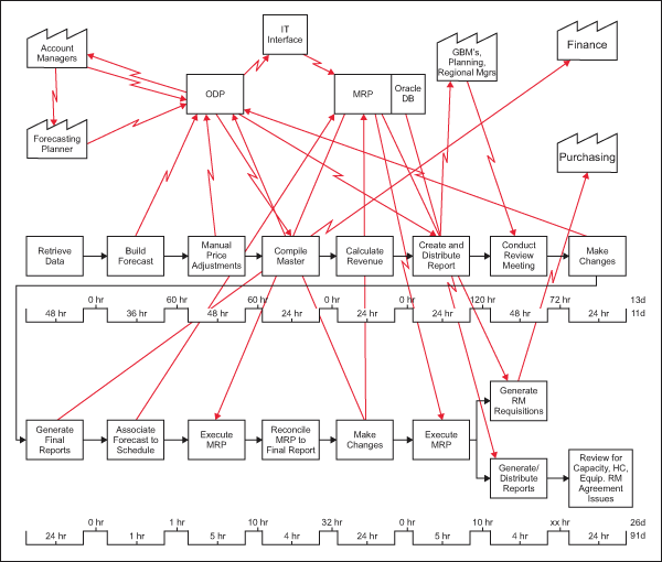
The perception of value for the process within the organization was very low. Measuring the process cycle time gave one indication why this condition existed. A process cycle time of 38 working days existed for a process that was performed every 45 calendar days. Figure 1 shows the basic value stream map of the process that shows the many data handoffs that occurred in this process.

Capability of this process to produce accurate forecast was equal to a Z score of zero. In real terms, the process was not capable of predicting volume to more than 50 percent accuracy. This supported the forecast accuracy metrics indicating approximately 40 percent accuracy was the historical average for the process. The project team realized that a new approach to forecasting was needed to make the significant improvement that leadership wanted. 

What’s Wrong with This Picture?

The team analyzed the process and determined that there were a couple of significant root causes for the current process performance. Those were: 

• No visibility into the end customer’s order drivers.
• No defined process ownership within the company.
• A slow painful process focused too much on extreme detail.

The issues around the process ownership and length of the process cycle time were largely management and administrative and were worked out through a series of meetings with the key stakeholders for each of those areas. The issues around gaining visibility to the end customers’ order drivers proved far more difficult to solve. 

At first he team attempted to build a model that would show what the expected order patterns of customers would be. The team put together a panel of company experts and together brainstormed possible factors that would influence customer ordering. From that, the team set off on the daunting task of gathering data on as many of those factors as possible to build a more complete model. While data was not available for every factor identified, the team felt that enough was present to justify some analysis. 

The team wanted to determine if a transfer function could be uncovered that would prove reliable in predicting order volume from customers. The team performed simple regression studies of the factors against the response of historical sales volume to determine if any combination of backward-looking factors could produce a sufficient explanation of the variation seen in order volume over time. Two things resulted from this work. First, though the team had some Predicted R2 (a measure of explanatory adequacy) values in 70-plus percent range, the actual accuracy against those predictions was poor. Secondarily, it proved very difficult to turn those factors with data from backward looking to forward predicting. Here is an example regression result for one particular region: 

HSV-Region 1 = 420930 – 156234 ICS-ALag6 + 665 SIS-Lag2 + 76651 DASI-Lag4 – 527840 DASI 

S = 20573.0 R-Sq = 86.0% R-Sq(adj) = 79.7% 

PRESS = 7766351996 R-Sq(pred) = 71.37%

 Missing Some Key Parts…

Concluded from these results was that even though the team had good predictive values, it was missing some key parts of the equation. Only after further analysis did the team discover that it had failed to consider a key piece of the process – specifically the field sales force. The team had been searching for a purely quantitative model to replace the current qualitative process; instead it should have supplemented the qualitative process using quantitative data as the starting point. This produced another problem. The team needed to determine how much value to assign to each part. The answer was found using principal component analysis (PCA) and regression. 

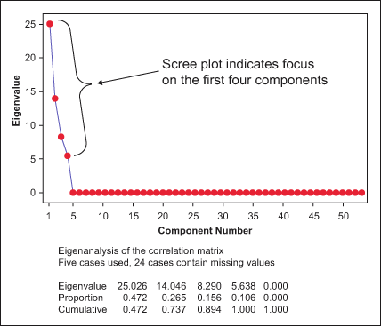
Principal component analysis is a method used to determine which of a group of factors has the most influence compared to other factors. PCA removes data duplication so that effective regression can be accomplished. Using PCA, the team was able to assign values for each segment of the transfer function based on the contribution of its representative factor to the overall explanation of variation in sales volume. Figure 2 shows the scree plot of the analysis followed by the data values. 

The Team’s Forecasting Improvements

The Transfer Function: Regression of the principal component representatives produced an R2 value of 91, significantly higher than any previous analyses. This also made the case for bringing in quantitative analysis of the overall market indicators provided by an outside firm specializing in statistical modeling of activity in the electronics industry. What these results told the team was that roughly 48 percent of the company’s variation in aales volume could be explained by variations in the end customers’ order drivers, while the remainder could be explained through our competitive situation or our customers’ competitive situation. 

The interesting twist in this study was that the p-values for most components were higher than the default cutoff of 0.05, which would traditionally discount their usefulness in explaining the variation. This was not a problem in this case, however, because the regression work was strictly a confirmation that the representative chosen as proxy’s for the principal components were meaningful to explaining overall response variation. The team had no intention of using the specific factors themselves to model variation in sales volume, only to understand the contribution of each area to the overall transfer function. 

Other improvements: With a better understanding of the process, the team was able to improve cycle time by eliminating non-value-added steps from the process (a traditional Lean approach to waste elimination) and driving accountability through process ownership. The process cycle time was reduced from 38 to 21 days, allowing the process to be performed monthly instead of every six weeks as it was previously. 

As a result of rolling out the new process improvements, overall improvement in process accuracy was 44 percent. 

Avoiding the Purist Mindset

The traditional DMAIC (Define, Measure, Analyze, Improve, Control) process and tools can be used to improve transactional and business processes, though their use may be in a non-traditional way. When working on transactional or business process improvements, it is best not to adopt a purist mindset regarding the application of the process and tools. One should search outside the traditional Six Sigma toolbox for other tools for process improvement, and understand the fundamental purpose of applying the tools used. A deeper understanding of why a particular toolset (such as regression or Lean) should be applied can enable a new view of the results and what they mean to the team, rather than a strict focus on the statistics.