During a Six Sigma project, the defect rate of the business process is calculated twice, first during the Define phase to show the impact of the problem and again during the Control phase to show how the process has improved. Although effective analysis of data that is not distributed normally is possible, completing one of the action steps below is beneficial for some projects to create a more useful data set:

• Divide the data into subsets according to business subprocesses.
• Mathematically transform the data and specification limits.
• Turn the continuous data into discrete data.

Process Capability

The goal of a process capability calculation is to use a sample of items or transactions from a business process to make a projection of the number of defects expected from the process in the long term. The defect rate, expressed as DPMO (defects per million opportunities), is part of the common language of Six Sigma. Expressing a business problem as a defect rate typically provides a more direct way to communicate with stakeholders and members of the project team.

The process capability calculation is based on:

1. The mean of the sample.
2. The standard deviation of the sample.
3. The known characteristics of the distribution.

The normal, or Gaussian, distribution is commonly observed in data involving a physical measurement of some kind such as length of machined bars, weight of widgets or the average number of manufacturing defects per week. It is less common in a transactional environment when tracking financial information or cycle time.

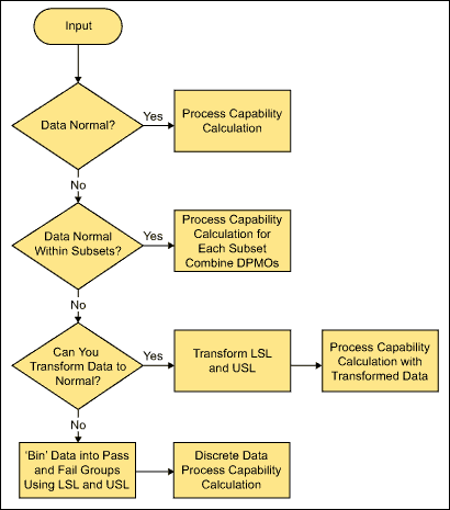
The flowchart in Figure 1 shows the logic of calculating the process capability starting with a set of continuous data. Note that the subsets referred to in the figure are not the small groups of transactions occurring in close increments of time used to estimate short-term process capability.

Process Capability with Subsets

In a typical business process, different subsets of transactions commonly pass through different parts of the business process. Large differences between subsets may cause baseline data to reflect as non-normal.

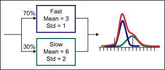
Figure 2 shows a process where 30 percent of the transactions proceed through a slower process than the majority of transactions. To account for this type of situation, subdivide the data into the individual processes, perform a process capability calculation on each subset and combine the DPMOs from each subset weighted by their relative percentages (Table 1). 

Transforming the Data

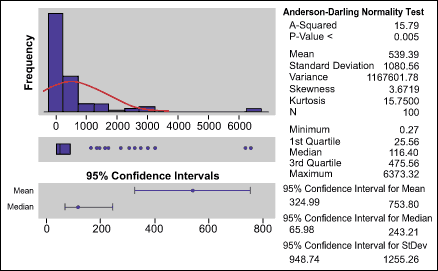
Different business processes may produce data with a non-normal, but well understood probability distribution. The example in Figure 3 represents a financial process where the defect definition is “whenever an order over $1,000 is processed without a valid letter of credit.” The graphical summary shows the data is highly skewed to the right.

Note the difference between the observed histogram and the curve representing a normal distribution curve. The process capability calculation would over-estimate the defect rate if the data were used in this form. 

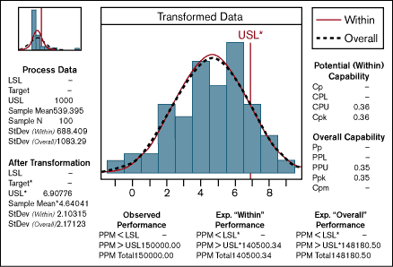
When data follows a well-known, but non-normal distribution, such as a Weibull or log-normal distribution, calculation of defect rates is accomplished using the properties of the distribution given the parameters of the distribution and the specification limits. An alternative approach is to mathematically transform the raw data into an approximately normal distribution and calculate the process capability using the assumption of normality and the transformed data and specification limits. Minitab provides the functionality to transform the raw data during the calculation of the process capability. The application transforms the specification limits at the same time and calculates the DPMO on the transformed data (Figure 4).

The upper left corner of Figure 4 shows a schematic of the calculation using the untransformed data. The main figure shows the good fit of the normal curve to the transformed data. The USL of $1,000 is simultaneously transformed to 6.9, producing a DPMO of 148,180. The process capability using the raw, untransformed data is 335,174 (Z = (1000-539)/1083 = 0.43), a 125 percent error. The number of defects or orders without letters of credit, is 15/100, producing a DPMO of 150,000, very close to the calculation of 148,180 using the continuous, transformed data. 

Turning Continuous Data into Discrete Data

When there are no identifiable subsets of transactions, or a method to transform the data into an approximately normal distribution, the best solution is to merely collect data on the defects themselves and summarize the results using discrete counts. This method has the disadvantage of preventing extrapolation beyond the sample at hand. To mitigate this issue, collect data samples that are much larger than is necessary with continuous data. 

Conclusion: Understand the Source of Non-Normality

When the data set reflects a non-normal distribution, it is helpful to understand the source of the non-normality. It may be caused by multiple and overlapping processes or by processes that generate data with well-understood, but non-normal data. When this occurs, transformation of the data will offer similar results for the process capability calculations done during both the Define and Control phases. The analysis here illustrates the effect on long-term process capability calculations. The logic in Figure 1 also applies to short-term process capability calculations.