The process capability indices P_p and C_p describe how closely a process can operate within its specification limits. Many articles describe the difference between P_p and C_p simply: one is short term, one is long term. Moving beyond such a description, this article focuses on the untapped power of capability analysis and shows you how to use P_p and C_p to your advantage.

Overview of P_p Versus C_p

The difference between P_p and C_p comes from the standard deviation that is used in the calculation.

When calculating P_p, the overall standard deviation is used. This is the standard deviation of all of the data combined, regardless of any subgroups in the data.

 P_p= (USL – LSL) / (6*σ_overall)

Where σ = standard deviation
USL = upper specification limit
LSL = lower specification limit

To calculate C_p, the within standard deviation is used.

 C_p= (USL – LSL) / (6*σ_within)

Notice on the sample Minitab output in Figure 1 that C_p is also known as the “potential” capability. You can gain a better understanding of what the process is telling you and what the process is truly capable of with this potential capability.

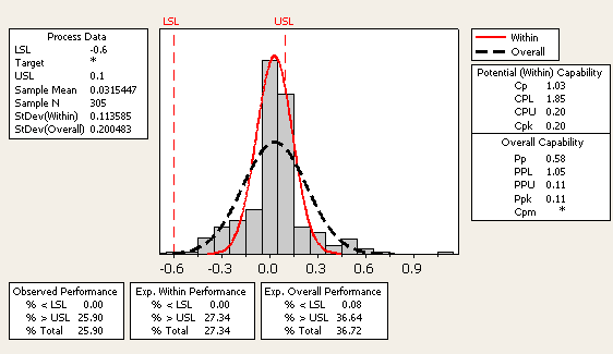
In Figure 1, the dotted black line represents the normal distribution of the data using the overall standard deviation of 0.20, while the red line represents the normal distribution of the data using the within standard deviation of 0.11.

Notice that P_p is 0.58 and P_pk is 0.11, while C_p is 1.03 and C_pk is 0.20. Given that P_p uses the overall standard deviation and C_p uses the within standard deviation, capability has the “potential” of going from 0.58 to 1.03, P_p to C_p respectively. Notice, too, that the defect rate would go from 36.72 percent to 27.34 percent – a potential reduction of 25 percent.

What is within capability and how is it calculated? The answer to this, like many questions regarding statistics, is, it depends. The within standard deviation is a function of the subgroup size that is used or chosen when the capability analysis is generated. This leads to the topic of subgroup size.

Subgroup Size Matters

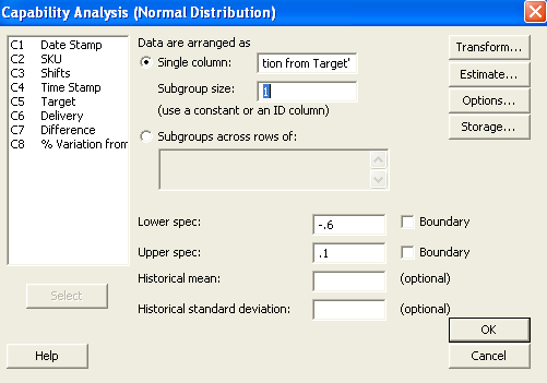
Many training instructors and materials default to using 1 as the subgroup size when teaching capability analysis. There is nothing wrong with using a subgroup size of 1 (Figure 2); however, it limits what you can learn about within variation and often overestimates the true potential capability.

The within standard deviation is based on the difference from one measurement to the next within a data set, akin to a moving range chart. The standard deviation is estimated from those differences. If, as is the case with a subgroup size of 1, the process has little variation from sample to sample (within) and a significant amount of variation through time (overall), you may see a capability analysis with a tall and skinny within/short-term/potential normal curve. The process capability shown in Figure 3 uses the same data as the initial capability analysis but this time with a subgroup size of 1.

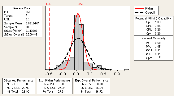
Figure 4 shows the same data using a subgroup size of 5.

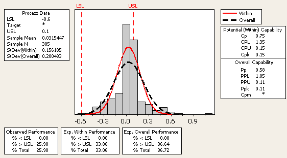
The overall standard deviation and resulting P_p does not change; it is not impacted by the subgroup size. However, the within standard deviation went from 0.1135 to 0.1561, thereby changing the C_p from 1.03 to 0.75.  The expected within performance went from a 27.34 percent defect rate to 33.06 percent, even though nothing has changed in the process. Again, the same data is used in each example.

The difference between the within standard deviation where n = 1 versus n = 5 is this: Using a subgroup size of 1 takes two consecutive points and calculates the difference, and the estimated standard deviation is calculated based on these differences. Because of this, it is important to remember that since the within standard deviation is using the moving range, the data must be in production order.  Otherwise, the within standard deviation calculation and resulting C_p will be incorrect.

Using a subgroup of 5 takes the standard deviation of 5 samples, then the next 5 samples, then the next 5 samples, etc., and estimates the within standard deviation.

Should you run your analysis using a subgroup size of 1 or 5? The subgroup size used for analysis must reflect how the data was collected. If you collected 5 measurements every hour then use a subgroup size of 5. If you collected individual samples over time, then your subgroup size is 1.

Getting More from Capability Analysis

Consider the capability analysis for a given Y variable, such as product variation from target, at various levels of an X variable, such as SKU (stock-keeping unit), instead of using a predetermined subgroup size. Rerunning the capability analysis using the X variable level as the subgroup (as shown in Figure 5) will lead to the results shown in Figure 6.

This is the same data used in the earlier capability analysis, but this data is sorted by the X variable. Doing so will yield a within standard deviation that is different than the capability results obtained when a subgroup size of 1 or 5 was used.

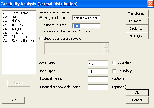
Analyzing the data with rational homogeneous subgroups instead of using a subgroup size of 1 will help answer the following question: What would the process capability be if all of the levels of the X variable were more alike, with the same average and the same standard deviation? In other words, what is the capability of the process if the variation between the X variable levels were eliminated?

In this case, the improvement would go from 0.58 (P_p) to 0.80 (C_p) and would have an overall average of 0.0315 and standard deviation of 0.146.

In conclusion, the within capability depends on your subgroup size.

Benchmark and Goal-setting Analysis

Capability analysis can be particularly useful for comparing the current process to another process, benchmark or project goal.

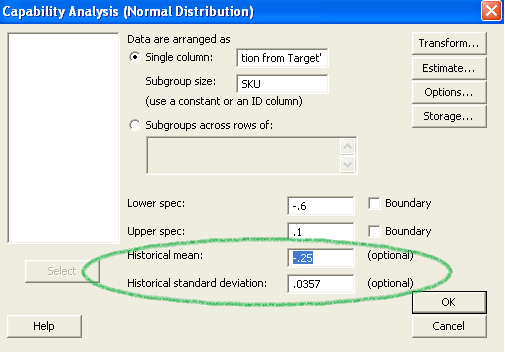
What is the potential capability at a predefined mean and standard deviation? This could be in regard to a particular SKU, a competitor’s product, a project goal, etc. Continuing with the same example, suppose the goal of the project is to center the process at -0.25 (centered between the upper and lower specification limits) and to reduce the standard deviation to that of SKU F, 0.0357 (Figure 5). With the “historical mean” and “historical standard deviation” options in the Minitab window (Figure 7) filled in, the results of the capability analysis are shown in Figure 8.

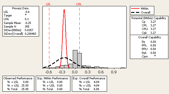
One notable difference is that the normal curves for both the within and overall process no longer represent the data.  The red curve represents the historical parameters (mean = -0.25, standard deviation = 0.0357) and overrides the within standard deviation from the data. The dotted black line is also centered on the historical average (-0.25) but maintains the overall standard deviation from the data.

This information can help determine what the process could look like if the average was centered and the variation reduced – that is, the potential capability of the process. For the example presented here, if the process was improved to the levels entered in the historical mean and historical standard deviation boxes, the process has the potential of going from a capability of 0.58 to 3.27. This knowledge can be used for project justification since the defect rate can be determined when target improvements for both the center and the variation are applied.

The Power of Capability Analysis

Capability analysis is an extremely powerful analytical tool and can be used for many applications. It is important to understand the within standard deviation and to know how a benchmark capability analysis can be used to determine a future state of the process.