
Resource utilization is managed using models. These models are created based on multiple influencing variables or factors. The goal is to balance resources – including people and skill levels – to achieve higher service levels, lower costs and other benefits.
Widely used across industries, resource modeling functions as an efficient decision-making tool. Some successful applications include the following:
- A retail organization recorded an annual savings of $52 million.
- A consulting firm increased its share of business by 35 percent.
- A call center raised productivity to 98 percent.
This article uses a hypothetical case within the field of information technology (IT) to show the mechanics for building these models. The reduction of time to provide a customer with information is the key process output variable, but there are others. The input variables will be discussed using an input-process-output (IPO) diagram and various analytical methods.
What Can Resource Modeling Do?
Deciding on the skill types for human resources as well as how many employees are needed during the initial set-up for a recently migrated process (moving a process from one computing platform to another) is a big challenge. This is especially true for resourcing decisions needed to create steady state operations. Lean Six Sigma tools and methods are useful for the stabilization and improvement of performance metrics, such as the time needed to respond to a customer issue, the time to resolve an issue and compliance with service-level agreements.
Resource modeling helps answer key questions such as:
- Which resource should be deployed?
- What are the constraints and the expected outcomes?
- Are the influencing factors interrelated?
- How should human resources be based – geography, skills or other factors?
- How can maximum productivity and efficiency be ensured?
- What is the optimum number of employees required to ensure timely response to customer inquiries?
- How can cost effectiveness be maximized?
Using LSS to resource modeling ensures a bias-free, precise and accurate outcome. It also helps create models based on multiple combinations of resource estimation, feasibility, control and simulation.
Example: Server Migration
The migration of multiple servers across the world is used as an example for resource modeling. The servers are the inputs or independent variables. The output time, in seconds, is the response variable. The resources to be modeled are employees.
The goal was to keep the output time to less than 60 seconds. The team collected information daily over a time period of six months for the output times (dependent variables or key process output variables [KPOVs]) and the several independent variables (key process input variables [KPIVs]) identified through brainstorming. This information was collected for three different locations. These are partially shown in the Minitab table in Figure 1.
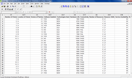
The first step for building a model was identifying the relevant variables thought to influence the output time. The IPO diagram shown in Figure 2 was used by the migration team to identify the variables of interest.
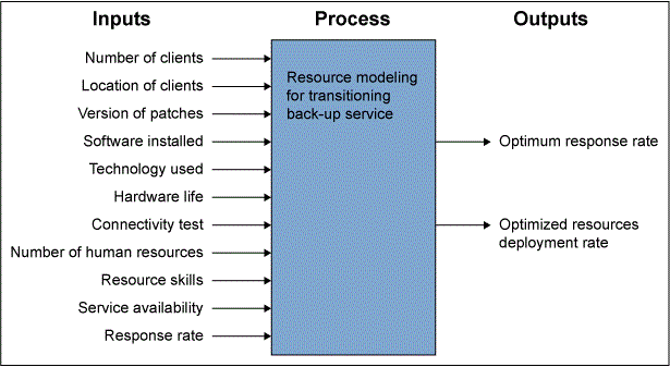
The second step for building the model was using exploratory data analysis including box plots and scatter diagrams to understand the relationships between the output time and the input variables. In the first analysis, shown in Figure 3, the combination of “location B, old technology, no software” appear to be potential KPIVs. In the second analysis, shown in Figure 4, the combination of “low skills (L1), no software, older software patch version” also appear to be potential KPIVs. Location may or may not be important for explaining variation in the output time. Connectivity testing does not appear to an important variable.
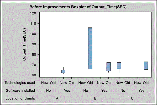
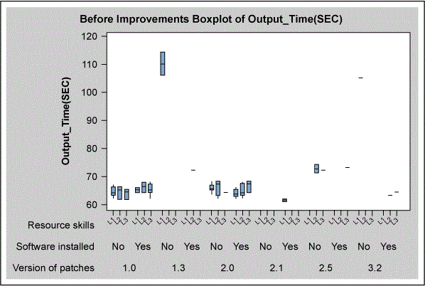
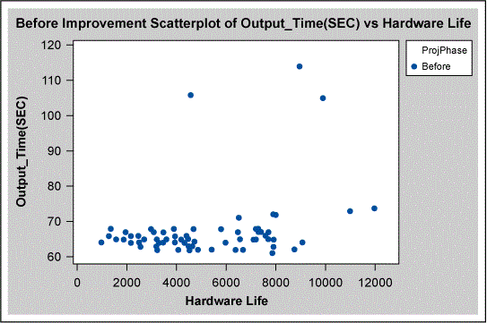
Hardware life (a continuous variable) was also analyzed, using the scatter plot shown in Figure 5. There is a great amount of variation in the graph, suggesting that hardware life is not important.
The team used stepwise regression to automatically exclude unimportant variables and include important variables to build a resource model relating output time to the various inputs identified using the IPO. Stepwise regression is an algorithm that builds a multiple linear regression model with only statistically significant KPIVs (e.g., having a p value less than 0.05). The algorithm started with all the input variables of the IPO. The important KPIVs or input variables appear to be Location B, certain software applications being installed and the higher skill level (L2) was used to answer customer inquiries. These variables have low p values, <0.05, indicating statistical significance. These are shown in the table below.
| Table 1: Response Is Output_Time (SEC) on 18 Predictors (N=151) | ||||
| Step | 1 | 2 | 3 | 4 |
| Constant | 6.660 | -6.845 | -10.785 | -8.898 |
| Location of Clients_B | 19.8 | 21.4 | 17.3 | 16.5 |
| T-value | 8.96 | 10.35 | 8.43 | 8.13 |
| P-value | 0.000 | 0.000 | 0.000 | 0.000 |
| Hardware Life | 0.00183 | 0.00187 | 0.00184 | |
| T-value | 5.09 | 5.65 | 5.69 | |
| P-value | 0.000 | 0.000 | 0.000 | |
| Software Installed_NO | 10.2 | 10.4 | ||
| T-value | 5.9 | 5.51 | ||
| P-value | 0.000 | 0.000 | ||
| Resource Skills_L2 | -4.9 | |||
| T-value | -2.60 | |||
| P-value | 0.010 | |||
| S | 12.8 | 11.9 | 10.9 | 10.7 |
| R2 | 35.01 | 44.70 | 53.56 | 55.61 |
The regression analysis explains about 54 percent of the variation of output time. In other words, 54 percent of output time can be explained by these KPIVs. The current model is:
Output time = -8.898 +16.5 (Location = B) + 0.00184 (hardware life) + 10.4 (if no software was installed) – 4.9 (if L2 skills were used)
Because the team wanted a higher R2 adjusted number – that is, 95 percent – the second phase of the analysis was modified to keep several variables constant. This included using the latest technology, software, the most current software patches, the higher skill sets (i.e., L2 and L3) and ensuring connectivity was established.
The reduced set of variables included in the stepwise regression model included the following: number of clients, hardware life, number of human resources and the location of clients. The resultant model shown in Figure 6 had an R2 term of 96 percent. The important variables were now location and number of clients.
| Table 2: Response Is Output_Time (SEC) on 6 Predictors (N=18) | ||
| Step | 1 | 2 |
| Constant | 52.67 | 51.75 |
| Location of Clients_B | 10.83 | 11.02 |
| T-value | 19.30 | 22.20 |
| P-value | 0.000 | 0.000 |
| Number of Clients | 0.142 | |
| T-value | 2.44 | |
| P-value | 0.027 | |
| S | 1.12 | 0.981 |
| R2 | 95.88 | 97.05 |
| R2 (adjusted) | 95.62 | 96.66 |
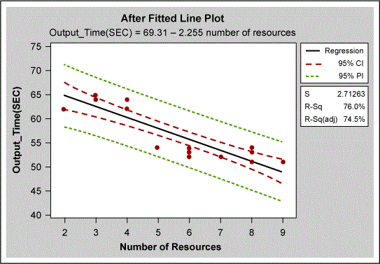
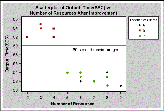
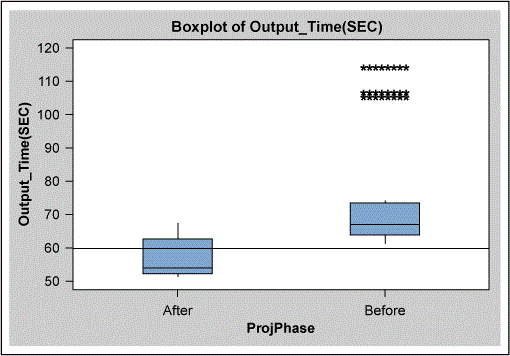
A suitable model was built using only “number of human resources.” The more detailed analysis shown in Figure 7 showed that the data set did not apply sufficient staffing to location B. The effect of this can also be seen in the “after” results in Figure 8, which shows that not all data points are below the 60-second goal. The problem at location B was corrected by ensuring that there were always six employees with L2 and L3 skills on each shift to keep the output time less than 60 seconds.
Summary
In summary, resource modeling helps to plan and determine the number of human resources required (here for an IT support project) to operate smoothly. It enables achieving the desired response rate and other targets efficiently. It also helps to lower operational costs and make key decisions about staffing levels in terms of numbers and skill levels. All help achieve an organization’s LSS goals.
Acknowledgment
A special thank you goes to James W. Martin for his valuable comments and encouragement as well as for sharing his knowledge.