Inspections are one of the most common methods of review performed in software teams. The goal of code inspection is to identify software faults early in the software development lifecycle. Teams are faced with the challenge, however, of determining whether those inspections are effective. One way to quantify this is by predicting the total number of faults that can be found in an inspection. A prediction model can be applied to evaluate an inspection process and refine the achieved quality level.
Inspection fault density (the number of operational faults detected divided by lines of code inspected) is used by development teams to evaluate the effectiveness of code inspections. Teams are required to re-inspect code wherever an inspection does not meet the inspection fault density guideline – which can potentially be a waste of resources. Alternatively, a block of code under inspection can be passed without trying to find (hidden, but existing) faults once the inspection fault density guideline is satisfied. Hence, there is a need for a fault prediction model based on various factors associated with software development and inspection. This article describes the development of such a model.
Prediction Model Foundation
The number of faults detected during code inspection is characterized by the Poisson distribution, which models counts of events having a constant mean arrival rate over a specified interval. The inspection model based on Poisson distribution assumes that the mean rate of fault introduction and fault detection is constant over a specified length of code block. In practice, however, there are several potential problems with this assumption:
- Different inspections generally cover code blocks of different lengths.
- The rates of fault introduction and detection probably vary over different coding languages. Other variables may also influence these rates.
- The fault detection rate will vary according to the inspector’s skill and preparation.
All of these problems are addressed by the statistical procedure called generalized linear modeling (GLM). Similar to regression, GLM is a response variable that depends on at least one continuous predictor and multiple categorical variables. This is a generalization of the Poisson model where the rate of detection also depends on other factors present in the model.
To develop a model that predicts the expected the numbers of faults to be found in an inspection, potential factors that influence fault detection need to be identified. Based on historical knowledge, the following eight potential factors were identified for further investigation:
- Type of inspected file: .c file / .h file / combination of both .c and .h
- Inspected size in lines of code (LOC): Formal inspections with greater than or equal to 40 LOC.
- Inspected size: This factor is considered to incorporate nonlinearity in the proposed model. It was observed that the number of faults detected follow a nonlinear trend with respect to the inspected size, or LOC.
- Type of work: Inspections done on a new feature (newly written code) or port feature (code taken from existing library).
- Complexity of inspected item: Essentially, this is a measure of the extent to which the code is prone to defects. As a measure of complexity, the average number of development and branches panic branches were used. (These are both types of revision control. A development branch is under development, not released officially and used to develop new features/modules. A panic branch is created when a change request is reported to rectify an operational fault in the system.) If a particular block of code has undergone frequent changes, then the probability of it being prone to defects is also high. Depending on the average numbers of development and panic branches, inspections were classified into one of three categories: 1) high-risk inspection (average of 10 development branches and average of 2 panic branches), 2) medium- risk inspection (average of 5 development branches and average of one panic branch) and 3) low-risk inspection (without any development and panic branches).
- Programming language: Inspections done on code written in C or C++ language.
- Development teams: Inspection carried out by Team A or Team B.
- Platform: Platform used to develop the software, such as C and D (technological platforms based on which software/user interfaces are developed).
Model Development
Hypothesis testing was carried out to determine the significance levels of the aforementioned factors. The results are shown in Table 1.
| Table 1: Hypothesis Testing Results for Potential Factors | |||
| Factors | Statistical Hypothesis | p-value | Conclusion |
| File Type (.h and .c file) | H0 : p.h = p.c H1 : p.h ? p.c |
0.045 | Statistically significant |
| Type of work (new and port) | H0 : pnew = pport H1 : pnew ? pport |
0.00 | Statistically significant |
| Programming language (C and C++) | H0 : pc = pc++ H1 : pc ? pc++ |
0.312 | Fail to reject null hypothesis |
| Development Teams (A and B) | H0 : pA = pB H1 : pA ? pB |
0.368 | Fail to reject null hypothesis |
| Platform (C and D) | H0 : pD = pD H1 : pD ? pD |
0.620 | Fail to reject null hypothesis |
| Where p* is the inspection fault density for the specified criteria | |||
Based on the hypothesis testing results, it was concluded that two factors – file type and type of work – have a significant effect on the faults detected in an inspection. Next a GLM model was developed, using the numbers of operational faults as the response variable. The results of the GLM model are shown in Table 2.
| Table 2: Parameter Estimates for GLM Model (Log Link Function) | |||||||
|
Parameter |
Estimate |
Standard error |
95% Wald Confidence Interval |
Hypothesis Test |
|||
|
Lower limit |
Upper limit |
Wald chi-square |
Df |
Significance |
|||
|
(Intercept) |
-0.108 |
0.5458 |
-1.178 |
0.962 |
0.039 |
1 |
0.843 |
|
[file =.c ] |
-0.656 |
0.4532 |
-1.544 |
0.233 |
2.093 |
1 |
0.048 |
|
[file =.c and.h] |
-0.46 |
0.4195 |
-1.282 |
0.362 |
1.202 |
1 |
0.023 |
|
[file = .h] |
0 |
||||||
|
[work = new] |
0.579 |
0.2607 |
0.068 |
1.09 |
4.928 |
1 |
0.026 |
|
[work = port] |
0 |
||||||
|
Inspected size |
0.003 |
0.0009 |
0.001 |
0.005 |
10.342 |
1 |
0.001 |
|
Inspected size squared |
-8.58E-07 |
4.37E-07 |
-1.72E-06 |
-1.31E-09 |
3.853 |
1 |
0.05 |
|
Average development branches |
0.03 |
0.0248 |
-0.019 |
0.079 |
1.441 |
1 |
0.03 |
|
Average panic branches |
0.288 |
0.4396 |
-0.573 |
1.15 |
0.43 |
1 |
0.012 |
| R2 adjusted = 60.03% | |||||||
Prediction Charts
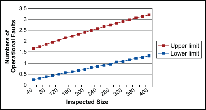
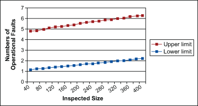
The results of the statistical analyses shown in Table 2 were used to generate prediction charts with 95 percent confidence limits. The upper and lower limits were calculated based on the parameter estimate of 95 percent Wald confidence interval shown in Table 2. Since the inspected file type, work type, average numbers of development branch and average numbers of panic branch are significant predictors of faults (from Table 2), two separate prediction charts for each combination of these factors were generated and are shown in Figures 1 and 2.


A similar inspection fault prediction chart may be plotted for different combinations of predictor variables based on the requirements of software development.
Model Validation
Model validation was done on inspections as an ongoing project. Based on the existing guidelines for inspection fault density, 28 inspections were found to be free of defects or bugs. The parameters of these 28 inspections were fed into the GLM model and seven inspections were selected for re-inspection. Development teams were able to find additional operational faults in four of these seven inspections. However, this model correctly identified 16 inspections as bug-free and saved approximately 200 staff hours, which was a significant improvement.
Future Work
This model predicts the expected number of faults based on the detection ability of teams so this is still a guideline. This guideline can be converted to goals by including the testing defects, which are simply faults that were not detected in inspection. The model explains around 60 percent of overall variation in the predicted operational faults. Improvements in variability can be obtained by adding more predictor variables such as inspection rate, preparation rate, team size and the experience level of the inspection team.