
Imagine you are the quality manager for a consumer electronics manufacturer. At the previous staff meeting, the CEO asked the management team for ideas that could help the company become more competitive and increase profits. It is now one month later. During the staff meeting, members of the marketing department present some research that shows a positive correlation between the length of the warranty period and new sales.
A random sampling of customers indicates sales could rise by 3.1 percent by increasing the warranty period from the current 180 days to 360 days – almost a full-year warranty (Table 1).
| Table 1: Projected Effect on Sales of Increasing Warranty | ||
| Warranty Period (Days) | Projected Annual Sales (Units) | Percent Change from Base Level |
| 180 | 100,000 | N/A |
| 210 | 100,300 | 0.30 percent |
| 240 | 100,790 | 0.79 percent |
| 270 | 101,400 | 1.40 percent |
| 300 | 101,810 | 1.81 percent |
| 330 | 102,250 | 2.25 percent |
| 360 | 103,100 | 3.10 percent |
The sales team’s forecast confirms there is sufficient market demand for the additional 3,100 annual units. Manufacturing feels comfortable handling the additional production output. At the end of the presentation, the recommendation from the three departments – marketing, sales and manufacturing – is to extend the warranty to a full year. Everyone feels comfortable with their decision, particularly because the average life of the product is, in fact, 364 days. The company president excitedly turns to you and asks, “What do you think?”
While the business scenario presented here may seem oversimplified, Six Sigma or quality professionals engaged in improving existing processes or designing new ones will likely face similar situations relating to warranties. By reviewing some key quality assurance concepts and tools – reliability, failure rate and product life history – that can be used during the DMAIC (Define, Measure, Analyze, Improve, Control) and DMADV (Define, Measure, Analyze, Design, Verify) processes, practitioners can allow for better business decisions regarding establishing appropriate product warranties.
Defining Warranty
In commercial and consumer transactions, a warranty is an obligation or guarantee that an article or service sold is as factually stated or legally implied by the seller. A warranty often provides for a specific remedy, such as repair or replacement, in the event the article or service fails to meet the warranty. A product’s warranty period can be established based on several factors, including:
- The industry standard for the product
- What the competition is offering
- The period of time during which some percentage of the products will still be functioning correctly
Reliability and Failure Rates
In layman’s terms, reliability is the assurance that a product will perform as intended. In quality assurance terms, reliability is the mathematical probability that a product will perform its intended function satisfactorily for a pre-determined period of time, assuming it is used in a normal and customary manner within the product’s specified environmental constraints.
Because reliability is a probability, it must have a value between 0 and 1, or 0 percent and 100 percent. Its actual numerical value will depend on how long the product is expected to last. For example, if a product is expected to last one year, it may have 95 percent reliability. This implies that 95 percent of the products will still be working after one year. If it is expected to last for two years, the same product may have a reliability of 75 percent. That is, 75 percent of the products will still be working after two years.
In order to mathematically compute a product’s reliability, practitioners need to understand the product’s average life expectancy, or mean life. A product’s mean life can be determined by testing a sample of products until every one of the products fail, and keeping track of exactly when each of the individual products failed. When the test is completed, the mean life (x-bar) can be determined by taking the average of the data collected. Another term used in reliability is the product’s failure rate. If the product’s failure rate is constant, then the failure rate is the reciprocal of the mean life:
Failure rate = 1/(x-bar)
The Product Life Cycle
When analyzing a product or component’s failure rate over time, three distinct periods emerge:
1. Burn-in (infant mortality) – Failures that occur almost immediately due to components that do not meet specifications or workmanship that is not up to standard. This period is also known as the infant mortality phase. The Weibull distribution is commonly used to determine when the infant mortality period is over. Reliability in the Weibull distribution is calculated as follows:
b
R = e-(t / x-bar)
where
e = logarithm having base e, where e is the constant 2.7183
t = time
x-bar = mean life
b = the Weibull shape parameter
2. Constant failure rate – Once the failures due to components and workmanship are eliminated, products enter the constant failure rate period. During this period, there are relatively few product failures. The exponential distribution can be used for making reliability predictions during this period. Reliability in the exponential distribution is calculated as follows:
R = e-(t / x-bar)
where
e = logarithm having base e, where e is the constant 2.7183
t = time
x-bar = mean life
3. Wear-out – This occurs at the end of a product’s normal life expectancy. As components begin to wear out, product failures occur more frequently until they are all burned out. The normal distribution is often used to determine reliability rates during this period. The formula for reliability is:
R = 1.0 – P, where
P = Probability from the Normal or Z table
The Z value is the measure of the distance in standard deviations of a sample from the average. The Z value can be calculated as follows:
Z = (x – µ)/ó, where
x = Data value (the value of interest)
ì = Average
ó = Standard deviation
When viewed as a composite over time, the shape of these distinct periods appears like a bathtub (Figure 1).
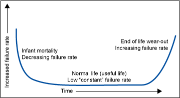
Knowing which period a component or product is in can help narrow down the nature of the failure and possible root causes (useful in the Analyze phase of DMAIC or DMADV). For example, failures occurring during the burn-in period can be considered quality-related issues, not design-related issues. Conversely, increasing failure rates that typically occur during the wear-out period are generally indicative of product fatigue. Understanding the nature of the failure can subsequently help shape and determine appropriate improvement or design strategies. As part of those strategies, the topic of warranties (type, length of time, etc.) will likely occur.
Calculating Reliability and Warranty Period
The following example illustrates warranty calculation: Based on 30 random product samples that were tested until failure, the average life of a sample product is 364 days (Table 2). Standard deviation is 18.09 days. This time frame reflects the wear-out period. Assuming a constant failure rate, the failure rate is 0.003 products per day [1/364].
| Table 2: Failure Rate of Product Samples | |||
| Sample | Failure Rate (Days) | Sample | Failure Rate (Days) |
| 1 | 360 | 16 | 355 |
| 2 | 370 | 17 | 364 |
| 3 | 330 | 18 | 398 |
| 4 | 361 | 19 | 375 |
| 5 | 345 | 20 | 338 |
| 6 | 364 | 21 | 366 |
| 7 | 385 | 22 | 322 |
| 8 | 370 | 23 | 365 |
| 9 | 358 | 24 | 360 |
| 10 | 385 | 25 | 372 |
| 11 | 345 | 26 | 365 |
| 12 | 361 | 27 | 365 |
| 13 | 340 | 28 | 385 |
| 14 | 390 | 29 | 355 |
| 15 | 386 | 30 | 385 |
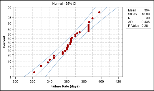
A probability chart (Figure 2) confirms the data to be normally distributed. The p-value is 0.281.
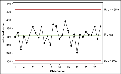
An individuals chart (Figure 3) reflects a process that is in control, hence, stable and predictable.
After a product’s mean life has been estimated, practitioners can compute the product’s reliability based on the appropriate distribution, depending on the life cycle. In this case, assume practitioners are interested in knowing the reliability of the product at 360 days. Accordingly, they would use the normal distribution to calculate the reliability.
Z = (360 – 364) / 18.09 = -0.221
The corresponding tail area of the curve is 0.4125 or 41.25 percent. The negative Z value indicates that the tail value is on the left tail of the normal curve (Figure 4). In other words, 41.25 percent of the products are projected to fail during the first 360 days. Correspondingly, 58.75 percent of the products should still be working at the end of 360 days.
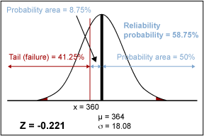
Based on these calculations, practitioners can quickly conclude that a warranty period of 360 days is unrealistic and would seriously erode profits and customer satisfaction.
An alternative approach to determine the appropriate warranty period might be to follow historical return rates. Say return rates for this product have never exceeded 0.25 percent of sales, and assume management decides they will accept this level for covered warranty repairs or replacements. Practitioners can use the Z table to determine the corresponding warranty period that will achieve a 0.25 percent return rate. From the table, they find the tail value of 0.0025. The corresponding Z value is 2.805. Because they are working on the left side of the mean, the Z value will be negative. The ideal number of warranty days can be calculated as follows:
Z = (x – µ) / ó
-2.805 = (x – 364) / 18.09
-2.805 x 18.09 = x – 364
x = 364 – 50.742
x = 313 days (rounded down)
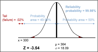
Therefore, if management sets a warranty period of 313 days, the company can expect no more than 0.25 percent of products returned for covered warranty repairs or replacement. Working together, the management team might ultimately decide on a 300 day warranty. Based on this warranty, only 0.02 percent of products are expected to fail at 300 days (Figure 5).
Balancing Revenue and Cost
Warranties are often used to help differentiate a company’s products and spur sales, but they can also have a profound impact on repairs or replacement costs and customer satisfaction. Accordingly, careful analysis should be performed that balances incremental revenues with warranty costs and customer satisfaction.