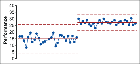
The DMAIC (Define, Measure, Analyze, Improve, Control) project lifecycle, the predominant methodology in Six Sigma for improving existing processes, is intended to bring about significant change in the behavior of the process under study. In order to know if such goals have been met, the process being worked on needs to be one in which performance can be measured in some tangible way. Figure 1 illustrates this concept by showing a process that went from predictably varying around an average of 15 to predictably varying – and varying less – around an average of 27.

For many processes that practitioners seek to improve, the preponderance of data is time-ordered data. The time order sequence of the data is an important contextual element that should be taken into account by the analysis. This requires a different type of analysis than might be used with a clinical trial or a political poll. With a time series, practitioners are not working with an existing population that could be enumerated; they are not extrapolating from a sample to a frame, but rather from the behavior in the past to behavior in the future. In his seminal work on curve-fitting, Some Theory of Sampling, statistician W. Edwards Deming said:

“In applying statistical theory, the main consideration is not what the shape of the universe is, but whether there is any universe at all. No universe can be assumed, nor the statistical theory of this book applied, unless the observations show statistical control. In this state the samples when cumulated over a suitable interval of time give a distribution of a particular shape, and this shape is reproduced hour by hour, day after day…In a state of control, the observations may be regarded as a sample from the universe of whatever shape it is. A big enough sample, or enough small samples, enables the statistician to make meaningful and useful predictions about future samples. This is as much as statistical theory can do.”¹

The fact that Deming included this in a book that explores how to fit various distributional models to data emphasizes its importance. In this one statement Deming essentially covers the relationships between all four of the basic questions of statistics.

The Four Questions of Data Analysis

The four questions of data analysis are related to:

• Description
• Probability
• Inference
• Homogeneity

Most statistics texts, and most classes aimed at teaching engineering or business statistics, do a fair job of covering the first three questions; most, however, do not address the fourth. An explanation of all four follows.²

Question One: Description

Given a collection of numbers, is there a meaningful way to represent all of the information in that collection using one or two summary values?

What is the median income in a state? What is the average SAT score for students in a local high school? What is the median price for a house in a neighborhood? What is the range of housing values in a neighborhood? All these questions are questions where descriptive statistics will provide summary values to judge and compare different sets of data.

The objective is to capture those aspects of the data that are of interest. Intuitive summaries such as totals, averages and proportions need little explanation. Other summaries that are less commonly used may require some explanation, and even some justification, before they make sense. In order to be effective in the end, a descriptive statistic has to make sense – it has to distill some essential characteristic of the data into a value that is both appropriate and understandable. In every case, this distillation takes on the form of some arithmetic operation:

Data + arithmetic = statistic

As soon as this is clear, it is apparent that the justification for computing any given statistic must come from the nature of the data itself – it cannot come from the arithmetic, nor can it come from the statistic. If the data is a meaningless collection of values, then the summary statistics will also be meaningless – no arithmetic operation can magically create meaning out of nonsense. An average phone number, for example, could be calculated, but what would be the point? The meaning of any statistic has to come from the context for the data, while the appropriateness of any statistic depends upon the intended use for that statistic.

Question Two: Probability

Given a known universe, what can be said about samples drawn from it?

How many royal flushes can be drawn from a regular deck of 52 playing cards? How many pairs when dealing out hands of five cards? How many sixes are likely to be rolled in 12 rolls of a fair die? How many odd values are there likely to be in 12 rolls?

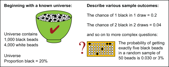
This is the world of probability theory: deductive logic, the estimation of possible outcomes and mathematical models. For ease of explanation, consider a universe that is a bowl filled with known numbers of black and white beads as shown in Figure 2. Then consider the likelihoods of various sample outcomes that might be drawn from this bowl.

When reasoning from a general situation, which is known, to descriptions of specific outcomes, which are presently unknown, practitioners are using an argument that is deductive in nature. Deductive logic proceeds from generalities to specifics and always has a correct answer. It is a process of reasoning in which a conclusion follows necessarily from the premises presented.

When starting with simple universes, such as beads in a bowl, it is often possible to list all possible outcomes. From these enumerations it is then possible to characterize the likelihood of different events. Since listing outcomes quickly becomes tedious, shortcuts are sought. By using probability theory, practitioners can develop mathematical models that allow the list-making step to be skipped – jumping directly from the known universe to the computation of the likelihood of different outcomes.

As mathematical models became increasingly sophisticated, and as methods of computing and approximating the probabilities progress, the models can be used to characterize more complex problems – problems that could never be handled by the enumeration approach. Thus, in probability theory practitioners are, in effect, playing a game – looking at the likelihoods of various outcomes drawn from a known universe so that this knowledge can be used later. At introductory levels, this game is restricted to homogeneous and fixed universes.

Before students can make much headway in probability theory, they need to be comfortable with deductive logic and mathematical models – two more elements of the foreign language of statistics. Fortunately, while probability theory is a necessary step in the development of modern statistical techniques, it is not a step that has to be mastered in order to analyze data effectively.

Question Three: Inference

Given a sample from an unknown universe, and given that everything about the nature of the sample is known, what can be said about the nature of the unknown universe?

If the average length of 10 pieces from an incoming lot of fabric swatches is 15.2 inches, is the average length of all the pieces in the lot 15.2 inches? How much error might there be in that estimate?

The problem here is the inverse of the probability question. What is known is only what is in the sample, but it is desirable to characterize the universe. To do this, the characteristics of the sample must be extrapolated to the characteristics of the universe – reasoning from the specific to the general. This is inductive logic. Unfortunately, all inductive logic is fraught with uncertainty. This is not a search for a single correct answer, but rather for a range of plausible answers; inductive logic cannot create certainty, only plausibility.

Statistical inference is built on inductive inferences. This is the realm of tests of hypotheses, confidence intervals and regression. These techniques permit the estimation of the parameters of the unknown universe (e.g., proportions, means and standard deviations). It is important to note that these estimates make sense only when the samples are all obtained from a single universe. This assumption of a single universe is equivalent to the assumption that the behavior of the outcomes in the sample is described by one probability model. Once this assumption is made, it is possible to use the probability model to characterize and predict the behavior of all the outcomes using the parameter values from the model.

Since the arguments of statistical inference are inductive, all of the estimates will have some amount of uncertainty built in. This is why good inferential techniques also characterize the uncertainty in the estimate. In order to do this, however, some assumptions must be made. The most critical assumption is that a given sample is being drawn from only one population or universe. If a sample is drawn from a lot that actually contains two or more different populations (e.g., pieces come from two or more different processes), all attempts to use descriptive statistics to estimate process characteristics flounder as there is more than one set of process characteristics present.

Statistical inference always begins with an assumption and ends with an indefinite statement. The assumption is that all the outcomes came from the same universe and the indefinite statement is couched in terms of interval estimates. If the assumption is incorrect, then none of the rigorous mathematical techniques in the statistical body of knowledge will lead to a useful or appropriate answer.

Question Four: Homogeneity

Given a collection of observations, is it reasonable to assume that they came from one universe, or do they show evidence of having come from multiple universes, processes or populations?

Descriptive statistics, probability models, and statistical inference all rely on homogeneity. An average is meaningless when the data comes from different universes. While an average can be computed, it does not describe any underlying property when the data is not homogeneous. Likewise, if there are multiple populations, there will also be multiple probability models. And inference is highly reliant on the assumption of homogeneity.

Before applying the techniques developed for answering the first three questions, the question of homogeneity must be addressed. Homogeneity can be assumed or evidence for homogeneity can be sought. In theory, assumptions are useful for the development of further theory. In practice, untested assumptions are dangerous. In practice, therefore, the assumption of homogeneity should be tested whenever possible before proceeding to deal with probability models, inference or descriptive statistics.

Why Proceeding with Caution Is Important

The four questions of data analysis are critical for data analysts everywhere. Lean Six Sigma practitioners are usually tasked with driving yields up, defect rates down, taking measurements to some desired level and reducing variation. To do that, there needs to be a starting point. What is today’s yield, defect rate or measurement? That starting point, articulated in project charters, is the baseline for a project. The baseline answers the descriptive statistics question related to the process under study. Since process steps tend to happen in sequence, they tend to generate time-ordered data. Time is an important context.

Consider a process example adapted³ from statistician Davis Balestracci’s original ASQ Statistics Division special publication “Data ‘Sanity.'”⁴

There are three clinics: A, B and C. “Daily proportion of nurse line calls answered within two minutes” is the selected metric. What can be said about the performance of the clinics, based on the histograms and data summaries shown in Figure 3?

These histograms all show reasonably symmetrical, bell-shaped data. The p-values for the Anderson-Darling tests for normality are all high, indicating no detectable departures from normality.

There are no apparent outliers. The average percentage for each clinic is a little over 84 percent and the standard deviation statistics are all around 2.6 percent. Are these three clinics alike? The use of the descriptive statistics implicitly assumes that each of these data sets is homogeneous. Unfortunately, Figure 3 does not provide any reliable way of checking for homogeneity.

How can homogeneity between the data sets be determined? The main tool for checking for homogeneity is the process behavior chart (also known as a control chart). Figure 4 shows the X chart for Clinic A.

In the case of Clinic A (where the histogram looked reasonably bell-shaped), the underlying process was changing over time. Can an average for all the data be calculated? Yes, but what does it represent? The average is not useful as a baseline because there is not one distribution, but many. The data is not homogeneous so the average does not characterize a process mean. The average does not represent where the process is today. There is no single value for the “true” process mean, so an observed average statistic does not generalize to represent anything useful about the underlying process.

Stating that the average of the pile of data represents the actual output is akin to saying that it is known where a hurricane is because the average latitude and longitude were calculated when it became a tropical storm off the coast of Africa – don’t worry about those high winds and heavy rains, Florida; on average, the storm is still only halfway across the Atlantic!

This leads to Clinic B (Figure 5). What is seen in the X chart in Figure 5 is three different universes; the process has shifted and stabilized three times. However, when the time order is ignored, the result is a pile of data that cannot be distinguished from data drawn from a single, normal distribution as seen in Figure 3.

Slicing the data for Clinic B at the shift points, as shown in Figure 6, illustrates that there are three distinct time periods when the process was operated predictably – three distinct cause systems were at work. The data shows up as stable performance over three periods of time. For the first 25 days, the process produced an average of 84.0 with natural process limits of 81.5 to 86.5. Then something happened and the process shifted. For the next 15 days, the average output was 81.2 with natural process limits of 78.5 to 83.8. Then the process shifted again, this time to average 87.1 with natural process limits of 83.5 to 90.8.

Note that the global average of 84.3 for Clinic B does not describe the location of this process on days 18 to 60 of this “baseline.” A lack of homogeneity will always undermine the ability to generalize from descriptive statistics to process characteristics.

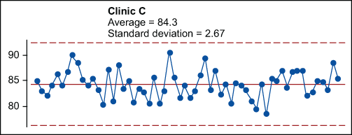
The only clinic with a stable process is Clinic C. Routine variation within the limits can be observed in Clinic C’s plot over time in Figure 7. The observed average of 84.3 characterizes the process mean. It can be predicted that, barring any deliberate process changes, this process will continue to produce daily values ranging from 76 to 92, while averaging about 84.

If the process is significantly drifting or shifting over time, such as is the case with Clinics A and B, a random sample across the shifts or changes will not result in a sample that can be used to represent the process. A random sample will lack the requisite homogeneity. While the descriptive statistics will still represent that “pile” of data, the pile of data will not represent the output of a single process with a single, well-defined mean and a single, well-defined standard deviation. Thus, the fault is not in the arithmetic, but in the incorrect assumption of homogeneity.

The Primary Question of Data Analysis

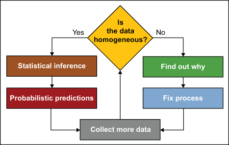
The primary question of data analysis is always the question of homogeneity. If the data is homogeneous, or once it has been organized into homogeneous groups, the techniques of statistical inference may be used to estimate parameters. Once there are estimated parameters, probability theory may be used to make predictions.

Given the structure of data, there will always be places within the data where the data is expected to be homogeneous. When the data fails to display homogeneity at these places the cause of the lack of homogeneity needs to be determined. When this happens there will be  something important waiting to be discovered. The lack of homogeneity presents an opportunity to fix the process. If the lack of homogeneity is ignored, the opportunity for improvement will be lost.

The Use of Good Judgment

In Six Sigma, practitioners are in the business of improving processes, improving the outcomes from processes, and improving the systems that produce products and services. Processes inherently produce data in time order, and some of the most important information in the data is tied up in this time order sequence. This is why judgment is an essential part of using process behavior charts.

When organizing data into subgroups, practitioners place two values together in the same subgroup based on a judgment that those two values were obtained under essentially the same conditions. When placing data on a chart for individual values, practitioners use judgment to assure that successive values are logically comparable. The chart has to compare apples to apples in order for the calculations to work as intended. Thus a judgment must be made that the values have, once again, been collected under what should be similar conditions. The name for this use of judgment is rational subgrouping.

Judgment plays a role as well in determining data collection frequency. The frequency has to make sense with respect to the process, to the understanding of how it changes, and the questions the resulting charts are intended to answer. The name for this use of judgment is rational sampling.

Additionally, when there is a physical boundary (such as zero for times or counts) and that boundary falls within the computed limits, judgment shows that the boundary takes precedence over the computed limit and the chart becomes one-sided.

Rational subgrouping and rational sampling (or good judgment) means that data cannot simply be placed on a chart in any old way. While there are situations where something other than the time order can be used, these situations still have to be based on context. Data cannot be placed on a chart in a random way. The data may be able to be shuffled to make an unpredictable process appear to be predictable; however, the shuffling of the data violates the requirements of rational sampling and rational subgrouping. If the requirement for rationality is ignored in terms of the context for the data, nonsense is likely to be the result. When this happens, it is not a failure of the technique, but a lack of understanding on the part of the user.

The Ultimate Goal Is to Take Action

The purpose of analysis is insight, and the reason for data collection is, ultimately, to take action. In an older paradigm, inspection was used with specifications to take action on items being inspected. The objective was to separate the acceptable outcomes from the unacceptable outcomes. Physician, statistician and engineer Walter Shewhart provided a better way to derive acceptable outcomes: study the process, look for assignable causes of variation and take action to improve the process so it will produce better outcomes in the future. To that end, he created process behavior charts to provide the insight needed when analyzing observational data and to provide a rational basis for prediction.

If taking action on a process is not planned, then nothing will be gained from process behavior charts. If, however, taking action on a process is desirable, process behavior charts are imperative for establishing a baseline and for detecting and evaluating the results of process improvement actions. Who knows, along the way a few assignable causes may be revealed and  some unanticipated ways may be unearthed to improve a process even before starting a project.

References

1. Deming, W. E. (1950). Some Theory of Sampling, pp 502-503, New York, NY: John Wiley & Sons, Inc.

2. Wheeler, D. J. (2005). The Six Sigma Practitioner’s Guide to Data Analysis. pp 1-11, Knoxville, TN: SPC Press.

3. Stauffer, R. F. (July 2013). Render unto enumerative studies. Quality Digest Daily. 31 July 2013. Retrieved from http://www.qualitydigest.com/inside/quality-insider-column/render-unit-enumerative-studies.html

4. Balestracci, D. (1998). Data “Sanity”: statistical thinking applied to everyday data. ASQ Statistics division Special Publication, Summer 1998, American Society for Quality. Retrieved from http://rube.asq.org/statistics/1998/06/data-sanity-statistical-thinking-applied-to-everyday-data.pdf