One branch of computational intelligence tools, neural networks, is worth surveying as part of the extended data mining and modeling toolkit. The focus here is on a specific kind of neural network applied to empirical model-building – comparing and contrasting its capabilities and performance to more traditional tools like regression analysis.
Neural Networks Mimic Biological Classification and Learning Systems
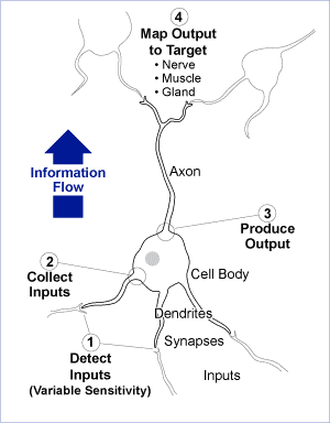
While neural nets are a mathematical construct, implemented in software, their history goes back to the early 1900s when researchers began trying to develop systems that mimicked the behavior they were coming to understand in the physiology of nerve cells (Figure 1).

Following the simple chain of events in a biological nerve cell provides a foundation for appreciating the math underlying computational nets. As illustrated in Figure 1, a biological nerve cell (1) detects excitation at its sensory structures called dendrites. A nerve cell body (2) collects inputs from the dendrites and, if they exceed a certain threshold, an electrochemical charge spike is sent (3) onto the output structure, the axon. This is referred to as the “firing” of a nerve. Nerve cells terminate in little buds, bordering a small liquid-filled gap, called a synapse, that touches either another nerve, a muscle or a gland. When the nerve buds are activated by firing, they produce chemical transmitters that diffuse across the thin synapse to, in turn, excite the nerve, muscle or gland on the other side (4). That simple structure is, of course, replicated into dense webs of nerves so that even simple living systems have much more than simple capabilities to react and adapt to situations in their environments.
While the biological neural mechanism is pretty simple, and slow (Table 1), even the most primitive living systems baffle supercomputers when it comes to adaptive behavior and learning. There must be something to the way they operate that enables an advantage even with the signal strength and speed limitations. Many agree that a key factor is the way they use “association” and parallel processing rather than “location” and linear processing.
| Table 1: Comparing Computational and Biological Systems | ||
|
Characteristics |
Nerve Cell Network |
Computer |
| Transmission speed | 101 to 102 meters/second | 2×10⁸ meters/second |
| Signal strength | Millivolts | Volts |
| Delay between pulses | Milliseconds | Nanoseconds |
| Information paradigm | Parallel processing/association | Linear processing/location |
Focusing on Software Backpropagation Networks for Modeling
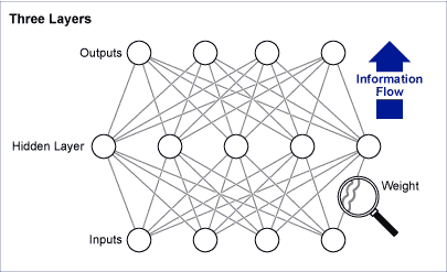
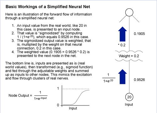
Efforts to build artificial neural nets started well before computers, with analog mechanisms that collected and fed signals through chains. An important notion early on was that adaptation and “learning” involved facilitating or inhibiting the excitation at the synapse connections. In software algorithms this became represented as weights that amplified or attenuated the numerical “signal” flowing on a neural path. From that base, network approaches for classification, signal processing and empirical model-building have evolved.
First attempts at neural models that learned from empirical data, auto-fitting themselves to a set of x-Y observations, were fairly crude. Actually, they topped out in a form that resembled regression. If the modeler could conceive the right model for an x-Y transfer function (including interactions and higher order terms) a network could be built to learn something like the transfer function through iterative training.

That was interesting, but did not bring any new capability to the toolkit. A breakthrough came with what is called “backpropagation” (Figure 2). All learning neural nets learn by comparing their current “prediction” (neural axon output) to a known right value (a Y). First answers are wrong, but the net can assess how wrong and in which direction.
Network weights are the variables that can be updated in a direction that reduces the error. Backpropagation uses calculus to attribute partial responsibility for the error to each weight, updating accordingly. The outcome is a net that can learn the equivalent of a complex regression model without the model-builder having to preconceive the form of the model. This does something that design of experiments and regression do not. It allows a simple construct of inputs (x‘s) to be mapped to one or more Ys. The net trains itself to find a minimum error mapping of those x‘s to each Y.
Backpropagation nets have been widely used in areas like material science and physics, where there are x-Y relationships, but their complexity and form are difficult to preconceive and express in basic regression terms.

Comparing and Contrasting Neural Backpropagation and Regression
A few key points can be illustrated with a simple example. In a software-controlled movement system, the states of four inputs (sensor 1, 2, motor 1, 2) are used to compute a movement correction signal – the Y (Table 2). The actual mechanism works like this: Sensors 1 and 2 provide input to movement control. Changes in motion depend on the speeds of two motors. After some oscillation, the right correction is known and written to a log file. A team wishes to use the correction data to improve the speed and accuracy of future corrections. Presently the correction signal is computed on the fly using an iterative algorithm. Researchers wonder if a model can be built allowing a transfer function to more quickly deliver the right Y answer.
| Table 2: Four Inputs, Correction Output and Comparison of Neural News and Regression Results Finding a Model | ||||||
|
Sensor 1 |
Sensor 2 |
Motor 1 |
Motor 2 |
Correction |
Neural Net |
Regression |
|
-0.97 |
0.10 |
0.35 |
-0.55 |
-237.41 |
-146.6 |
-25.3 |
|
-0.97 |
-0.28 |
-0.34 |
-0.71 |
-595.85 |
-721.8 |
-764.8 |
|
-0.94 |
0.98 |
0.62 |
-0.76 |
626.72 |
444.8 |
1013.1 |
|
-0.91 |
-0.58 |
-0.21 |
-0.59 |
-633.49 |
-760.2 |
-990.4 |
|
-0.80 |
0.75 |
0.85 |
0.56 |
1285.51 |
1344.5 |
886.0 |
|
-0.72 |
0.00 |
0.76 |
-0.06 |
1153.06 |
725.2 |
137.1 |
|
-0.67 |
-0.01 |
0.41 |
0.90 |
-959.62 |
-1137.9 |
-88.5 |
|
-0.56 |
-0.78 |
0.35 |
0.86 |
-1331.05 |
-1336.7 |
-864.6 |
|
-0.51 |
-0.32 |
-0.08 |
-0.81 |
-1061.91 |
-880.0 |
-552.7 |
|
-0.49 |
-0.21 |
-0.11 |
0.37 |
-207.63 |
39.3 |
-510.3 |
|
-0.43 |
0.28 |
0.29 |
0.81 |
-854.13 |
-796.1 |
196.9 |
|
-0.39 |
-0.58 |
0.15 |
-0.93 |
-1498.29 |
-1060.2 |
-665.4 |
|
-0.31 |
0.02 |
0.47 |
0.05 |
431.70 |
649.5 |
84.1 |
|
-0.29 |
-0.41 |
-0.40 |
-0.58 |
-270.25 |
-757.2 |
-771.9 |
|
-0.29 |
-0.40 |
-0.33 |
0.48 |
-212.88 |
-480.6 |
-770.8 |
|
-0.26 |
-0.20 |
0.75 |
0.47 |
756.47 |
595.9 |
19.6 |
|
-0.24 |
0.33 |
-0.48 |
-0.09 |
483.59 |
389.9 |
-96.0 |
|
-0.19 |
0.93 |
0.58 |
-0.44 |
1016.05 |
932.6 |
1105.0 |
|
-0.15 |
0.74 |
0.23 |
-0.80 |
590.27 |
-232.4 |
748.9 |
|
-0.07 |
0.92 |
0.96 |
0.11 |
2434.15 |
2251.9 |
1296.9 |
|
0.11 |
-0.95 |
0.19 |
0.04 |
-609.83 |
-443.0 |
-921.4 |
|
0.19 |
-0.73 |
-0.07 |
0.73 |
-1161.97 |
-1105.4 |
-853.7 |
|
0.61 |
-0.04 |
0.28 |
0.80 |
-860.49 |
-1071.7 |
114.2 |
|
0.73 |
-0.75 |
-0.04 |
0.48 |
-710.70 |
-400.1 |
-721.5 |
|
0.77 |
0.19 |
-0.54 |
-0.06 |
588.23 |
19.7 |
-23.1 |
|
Predictions (R-Squared) |
0.93013 |
0.51584 |
||||
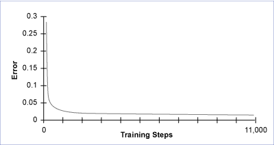
A neural network trained on the data in Table 2, begins with a random set of weights, and lots of error. Error drops and levels off during neural net training (Figure 4).

Putting regression at a bit of a disadvantage to make a point, assume that there is no real notion of what the right x-Y model should be. Linear regression, using just the four x’s, does not find a very good fit to the data – R-squared about 51 percent (Table 2). After training, the neural net predictions show a “goodness of fit” R-squared of about 93 percent.
Noting Neural Net Limitations
At first reading, the performance of a trained network, given a no-preconceived-model challenge with regression analysis, appears to work very well. This can be true – but some limitations need to be pointed out.
1. Neural nets do not deliver a human-readable transfer function. If the weights in the trained net that did so well in Table 2 (R-squared 93 percent versus 51 percent for regression) are examined, no human sense can be made of them. Their meaning is so buried in the sigmoidization and summing at nodes that they do not do anything like the coefficients in a regression transfer function to inform human engineering insight about what is going on. A net is truly a black box, albeit a very capable one.
2. A network model is not unbiased. In regression the sum of errors is zero and the sum of squared errors is minimum. This is important, as all models are unbiased – centered in the estimating space. A neural net starts with some random error and iteratively reduces it through training. Where it ends up has no relation to being unbiased. The sum of errors will likely be small, but with no guarantee that the model is not skewed.
3. Nets are prone to overfitting. Build a complex enough net and train it long enough and it will fit any arbitrary Y data. Just as regression models can be overfit (using up too much of the data degrees of freedom in the model itself – leaving little or none to estimate error), a neural net can “marry” a data set, reproducing it faithfully, but performing poorly in new predictions. There are approaches to manage this risk, generally involving holding back some data from the training set and using it as an error check for new predictions. This caution needs to be underlined, as people newly enthused about net modeling can get carried away with the goodness-of-fit indicators.
Conclusion: A Few Key Points
After a very short dip into a large subject pool, here are a few key points:
- Neural nets mathematically mimic biological nerve structures, treating adaptation and learning as an iterative update of node-to-node numerical weights.
- Backpropagation nets can find arbitrarily complex mappings of any number of x‘s to any number of Ys (in one model).
- Backpropagation learning involves iterative error assessments and smart weight adjustments to reduce error.
- Nets can do very well fitting data – so well that experimenters must be careful to remember that prediction performance on new data is of greater practical importance than fitting to a single data set.
- As net models are not unbiased, experimenters should look at residuals and understand if a particular model is significantly skewed.
- Neural models can be helpful when a) The form of a model is not known and may be complex (nonlinear, higher order terms, etc.), and b) There is value in a black box transfer function that can be updated on the fly (through further training on the updated x‘s and Ys).