© Ground Picture/Shutterstock.com
Key Points
- A Box-Cox Power Transformation allows you to transform data to match a normal distribution.
- It is not a guarantee of normality.
- It is a quick way of transforming data to better fit a control chart.
Normally distributed data is needed to use several statistical analysis tools, such as individual control charts, Cp/Cpk analysis, t-tests, and analysis of variance (ANOVA). When data is not normally distributed, the cause for non-normality should be determined and appropriate remedial actions should be taken. (An introduction to remedial actions for non-normal data can be found in “Dealing with Non-normal Data: Strategies and Tools.”)
Data transformation, and particularly the Box-Cox power transformation, is one of these remedial actions that may help to make data normal. By understanding both the concept of transformation and the Box-Cox method, practitioners will be better prepared to work with non-normal data.
What Are Transformations?
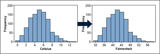
Transforming data means performing the same mathematical operation on each piece of original data. Some transformation examples from daily life are currency exchange rates (e.g., U.S. dollar into Euros) and converting degrees Celsius into degrees Fahrenheit.
These two transformations are called linear transformations because the original data is simply multiplied or divided by a specific coefficient or a constant is subtracted or added. However, these linear transformations do not change the shape of the data distribution and, therefore, do not help to make data look more normal (Figure 1).
What is the Box-Cox Power Transformation?
The statisticians George Box and David Cox developed a procedure to identify an appropriate exponent (Lambda = l) to use to transform data into a “normal shape.” The Lambda value indicates the power to which all data should be raised. To do this, the Box-Cox power transformation searches from Lambda = -5 to Lamba = +5 until the best value is found. Table 1 shows some common Box-Cox transformations, where Y’ is the transformation of the original data Y. Note that for Lambda = 0, the transformation is NOT Y0 (because this would be 1 for every value) but instead the logarithm of Y.
| Table 1: Common Box-Cox Transformations | |
| l | Y’ |
| -2 | Y-2 = 1/Y2 |
| -1 | Y-1 = 1/Y1 |
| -0.5 | Y-0.5 = 1/(Sqrt(Y)) |
| 0 | log(Y) |
| 0.5 | Y0.5 = Sqrt(Y) |
| 1 | Y1 = Y |
| 2 | Y2 |
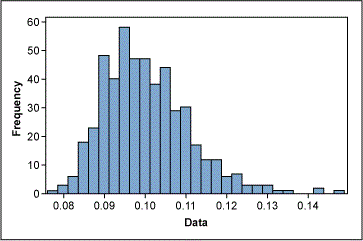
An example: Figure 2 shows non-normally distributed cycle time data. Using the Box-Cox power transformation in a statistical analysis software program provides an output that indicates the best Lambda values (Figure 3).
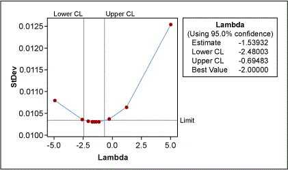
The lower and upper confidence levels (CLs) show that the best results for normality were reached with Lambda values between -2.48 and -0.69. Although the best value is -1.54 (estimate in Figure 3), the process works better if this value is rounded to a whole number; this will make it easier to transform the data back and forth.
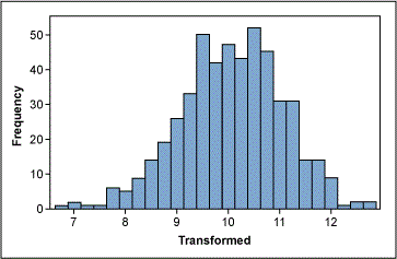
The best whole-number values here are -1 and -2 (the inverse function of Y and Y2, respectively). The histogram in Figure 4 shows the transformed data using Lambda = -1, now more normally distributed.
Does Box-Cox Always Work?
The Box-Cox power transformation is not a guarantee for normality. This is because it does not check for normality; the method checks for the smallest standard deviation.
The assumption is that among all transformations with Lambda values between -5 and +5, transformed data has the highest likelihood – but not a guarantee – to be normally distributed when the standard deviation is the smallest. Therefore, it is necessary to always check the transformed data for normality using a probability plot.
Additionally, the Box-Cox Power transformation only works if all the data is positive and greater than 0. This, however, can usually be achieved easily by adding a constant (c) to all data such that it all becomes positive before it is transformed. The transformation equation is then:
Y’ = (Y+C)l
Why It Matters
Statistical analysis is one of the most crucial parts of any project. However, what happens when your data doesn’t conform to the ideals set throughout a project? Given how much of statistical analysis relies on the assumption of a normal distribution, the Box-Cox power transformation is a powerful tool to get your data back on track.
Application Example
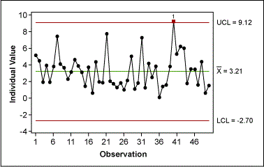
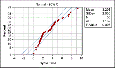
A project team collected cycle time data from a purchase order-generation process. One team member created a control chart of this data (Figure 5) and was about to ask what special cause had happened for data point 40 when the Green Belt remembered that using an individual control chart requires normally distributed data. A look at the probability plot of the data (Figure 6) revealed a non-normal distribution. Therefore, the control limits of the control chart were useless.
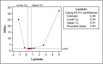
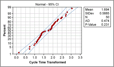
The Green Belt used the Box-Cox power transformation to determine whether the data could be transformed (Figure 7). Box-Cox suggested a best Lambda value of 0.5 for transformation (i.e., the square root of the original data). And the transformation worked: The new probability plot confirms normality (Figure 8).
Putting It Together
After the transformation, the Green Belt created a control chart of the transformed data and showed that the purchase order-generation process was quite stable, i.e., all variation was due to common causes (Figure 9).
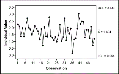
Because the individual values of the transformed data have no practical meaning, the Green Belt had to re-create a control chart for the original data, but this time with the correct control limits (Figure 10). To do this, the Belt used the upper and lower CLs from the control chart of the transformed data and transformed them back into their original values. Because the transformation operation was taking the square root, the back-transformation involved squaring the transformed data:
UCL = UCL’2 = 3.4422 = 11.847
LCL = LCL’2 = -0.0542= 0.003
For the mean, the Belt used the mean of the original data.
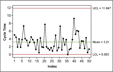
This control chart could then be used for the ongoing monitoring of the purchase order generation process.
Other Useful Tools and Concepts
While we’ve discussed this concept at length, there is still more to learn. How do you deal with non-normal data? This concept can leave many in the lurch, but thankfully, we’ve got just what you need when considering your toolbox and strategies.
Cox-Box isn’t the only thing at your disposal when it comes to transforming non-normal data. Our guide on how to compensate and transform said data is a great read and will have you on the fast track to success.
The image featured at the top of this post is ©Ground Picture/Shutterstock.com.
