
When conducting the 2-sample t-test to compare the average of two groups, the data in both groups must be sampled from a normally distributed population. If that assumption does not hold, the nonparametric Mann-Whitney test is a better safeguard against drawing wrong conclusions.
The Mann-Whitney test compares the medians from two populations and works when the Y variable is continuous, discrete-ordinal or discrete-count, and the X variable is discrete with two attributes. Of course, the Mann-Whitney test can also be used for normally distributed data, but in that case it is less powerful than the 2-sample t-test.
Uses for the Mann-Whitney Test
Examples for the usage of the Mann-Whitney test include:
- Comparing the medians of manufacturing cycle times (Y = continuous) of two different production lines (X).
- Comparing the medians of the satisfaction ratings (Y= discrete-ordinal) of customers before and after improving the quality of a product or service.
- Comparing the medians of the number of injuries per month (Y = discrete count) at two different sites (X).
Project Example: Reducing Call Times
A team wants to find out whether a project to reduce the time to answer customer calls was successful. Time is measured before and after the improvement. A dot plot (Figure 1) of the data shows a lot of overlap between the lead times – it is hard to tell whether there are significant differences.
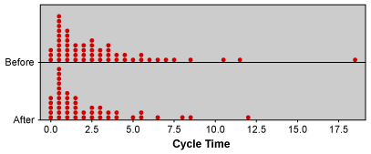
Therefore, the team decides to use a hypothesis test to determine if there are “true differences” between before and after. Because the data is not normally distributed (p < 0.05) (Figure 2), the 2-sample t-test cannot be used. The practitioners will use the Mann-Whitney test instead.
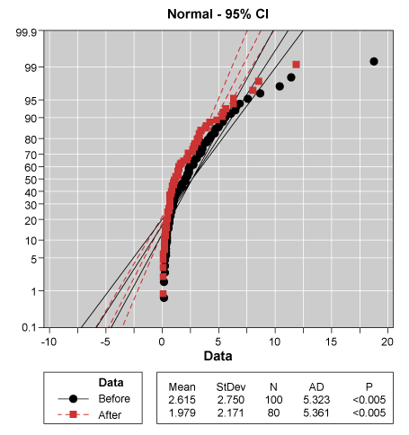
For the test, the null hypothesis (H0) is: The samples come from the same distribution, or there is no difference between the medians in the call times before and after the improvement. The alternative hypothesis (Ha) is: The samples come from different distribution, or there is a difference.
Passing Mann-Whitney Test Assumptions
Although the Mann-Whitney test does not require normally distributed data, that does not mean it is assumption free. For the Mann-Whitney test, data from each population must be an independent random sample, and the population distributions must have equal variances and the same shape.
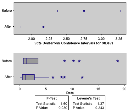
Equal variances can be tested. For non-normally distributed data, the Levene’s test is used to make a decision (Figure 3). Because the p-value for this test is 0.243, the variances of the before and after groups used in the customer call example are the same.
Ideally the probability plot can be used to look for a similar distribution. In this case, the probability plot (Figure 4) shows that all data follows an exponential distribution (p > 0.05).
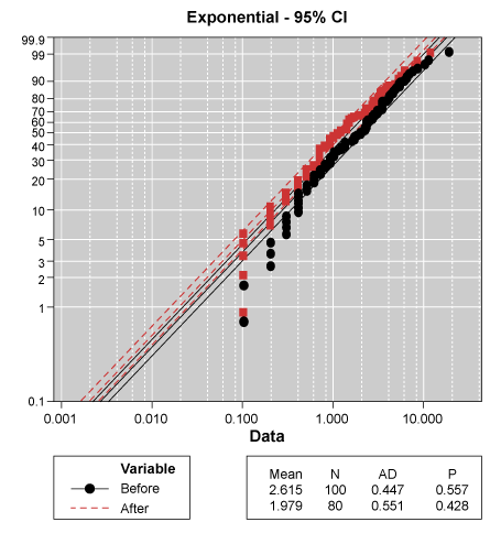
If the probability plot does not provide distribution that matches all the groups, a visual check of the data may help. When examining the plot, a practitioner might ask: Do the distributions look similar? Are they all left- or right-skewed, with only some extreme values?
Completing the Test
Because the assumptions are now verified, the Mann-Whitney test can be conducted. If the p-value is below the usually agreed alpha risk of 5 percent (0.05), the null hypothesis can be rejected and at least one significant difference can be assumed. For the call times, the p-value is 0.0459 – less than 0.05. The median call time of 1.15 minutes after the improvement is therefore significantly shorter than the 2-minute length before improvement.
|
|||||
How the Mann-Whitney Test Works
Another name for the Mann-Whitney test is the 2-sample rank test, and that name indicates how the test works.
The Mann-Whitney test can be completed in four steps:
- Combine the data from the two samples into one
- Rank all the values, with the smallest observation given rank 1, the second smallest rank 2, etc.
- Calculate and assign the average rank for the observations that are tied (the ones with the same value)
- Calculate the sum of the ranks of the first sample (the W-value)
Table 1 shows Steps 1 through 4 for the call time example.
| Table 1: Sum of the Ranks of the First Sample (the W-value) | |||
| Call time | Improvement | Rank | Rank for ties |
| 0.1 | Before | 1 | 4 |
| 0.1 | Before | 2 | 4 |
| 0.1 | After | 3 | 4 |
| 0.1 | After | 4 | 4 |
| 0.1 | After | 5 | 4 |
| 0.1 | After | 6 | 4 |
| 0.1 | After | 7 | 4 |
| 0.2 | Before | 8 | 11 |
| 0.2 | Before | 9 | 11 |
| 0.2 | Before | 10 | 11 |
| 0.2 | After | 11 | 11 |
| 0.2 | After | 12 | 11 |
| 0.2 | After | 13 | 11 |
| 0.2 | After | 14 | 11 |
| … | … | … | … |
| 7.5 | Before | 173 | 173 |
| 8 | After | 174 | 174 |
| 8.5 | After | 175 | 175 |
| 8.6 | Before | 176 | 176 |
| 10.3 | Before | 177 | 177 |
| 11.3 | Before | 178 | 178 |
| 11.9 | After | 179 | 179 |
| 18.7 | Before | 180 | 180 |
| Sum of ranks (W-value) for before | 9,743.5 | ||
Because Ranks 1 through 7 are related to the same call time of 0.1 minutes, the average rank is calculated as (1 + 2 + 3 + 4 + 5 + 6 + 7) / 7 = 4. Other ranks for ties are determined in a similar fashion.
Based on the W-value, the Mann-Whitney test now determines the p-value of the test using a normal approximation, which is calculated as follows:

where,
W = Mann-Whitney test statistics, here: 9743.5
n = The size of sample 1 (Before), here: 100
m = The size of sample 2 (After), here: 80
The resulting ZW value is 1.995, which translate for a both-sided test (+/- ZW) and a normal approximation into a p-value of 0.046.
If there are ties in the data as in this example, the p-value is adjusted by replacing the denominator of the above Z statistics by
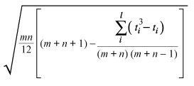
where,
i = 1, 2, …, l
l = The number of sets of ties
ti = The number of tied values in the i-th set of ties
The unadjusted p-value is conservative if ties are present; the adjusted p-value is usually closer to the correct values, but is not always conservative.
In this example, the p-value does not vary dramatically through the adjustment; it is 0.0459. This indicates that the probability that such a ZW value occurs if there are actually no differences between the call times before and after the improvement is only 4.59 percent. With such a small risk of being wrong, a practitioner could conclude that the after results are significantly different.